Data Preparation in the Graphical User Interface
< Previous section Next section >
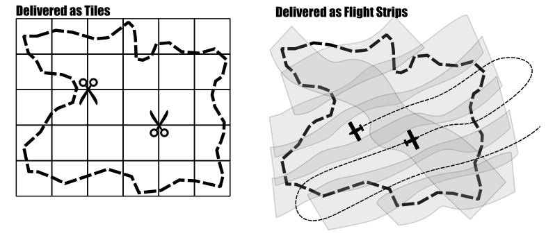
In this tutorial you will learn how to prepare your data for efficient processing and data access. Point clouds based on airborne laserscanning (ALS) are often delivered as individual files (either tiles representing some kind of regular grid; or overlapping flight strips). As LiDAR Data Analysts we want to handle the given dataset seemlessly as one single dataset (ignoring the given delivery structure).
In this tutorial section, we will prepare two neighbouring point cloud files for seamless (i.e., tile-independent) data access and processing. This is strictly required for large-scale processing (meaning tens to hundreds or thousands of such point cloud files), but also simplifies processing even in the case of just two tiles!
Make sure you have setup the folder structure as described in the previous section:
AUTOMATION_GUIDE
├── data
|   ├── 472053_5245903.laz
|   └── 472053_5245153.laz
└── processing
    ├── export
    ├── shapes
    └── spc_class
Now open the LIS Pro 3D Graphical User Interface (GUI)!
Create a New Project
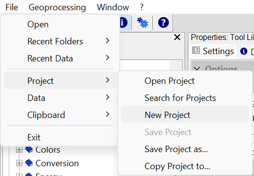
If you have any data open in LIS Pro 3D, open a new clear project (File > Project > New Project)!
We recommend creating a SAGA GIS project when starting a new workflow. Regularly saving the project and any processed data (vector and raster datasets, as well as point clouds) can also be very helpful.
Create LAS/LAZ Index
This helps to query subsets of a laz-file faster. Use the tool Create LAS/LAZ Index!
- Provide all available LAS/LAZ-files as Input Files
- Click Execute
This will create spatial indices for the input LAZ files to speed up spatial queries later!
Tool: Create LAS/LAZ Index
Geoprocessing: LIS Pro 3D → Import/Export → LAS/LAZ // Tools → LIS Pro 3D → Import/Export
| Parameter | Setting |
|---|---|
| Input Files | “/…/data/las/472053_5245903.laz” “/…/data/las/472053_5245153.laz” |
| Input File List | |
| Index All Files | 🗹 |
| Indexing | |
| Tile Size | 0 |
| Threshold | 1000 |
| Adaptive Coarsening | |
| Minimum Point Count | 100000 |
| Maximum Interval Count | -20 |
Create a Point Cloud Catalog
Create a point cloud catalog for the laz files by running Create Virtual LAS/LAZ Dataset. The catalog references all the individual point clouds. We can work with the catalog as if it would be one single file that contains all of the points (despite only having a reference to the real files!).
- Provide all available LAS/LAZ-files as Input Files
- Define an output *.lasvf-file (put it into the location of the laz files)
- Click Execute
Tool: Create Virtual LAS/LAZ Dataset
Geoprocessing: LIS Pro 3D → Virtual → LAS/LAZ // Tools → LIS Pro 3D → Virtual
| Parameter | Setting |
|---|---|
| Input Files | “/…/data/las/472053_5245903.laz” “/…/data/las/472053_5245153.laz” |
| Input File List | |
| Filename | /…/data/las/tiles.lasvf |
| File Paths | relative |
| Color Depth | 16 bit |
| Riegl Extra Bytes | ☐ |
| Ignore LAS File Version | ☐ |
| Ignore Point Data Record Format | ☐ |
| Ignore Coordinate Reference System | ☐ |
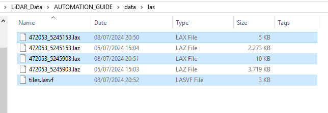
As a result of the previous two tool calls, we now have a laz-index file for each laz-file (ending on “.lax”) and a single virtual las file (the “catalog”, ending on “.lasvf”) in the data folder:
Create Vector Layer Showing the Bounding Boxes of Your Input Data
Now, we will create a vector layer that contains the bounding boxes (a polygon) that describe the outlines of each laz-file in the virtual las-file (*.lasvf). This will help to get an overview of how your data is laid out initially, before processing. Use LIS Pro 3D > Virtual > Create Tileshape from Virtual LAS/LAZ.
- Provide the *.lasvf file as Filename
- Click Execute
Tool: Create Tileshape from Virtual LAS/LAZ
Geoprocessing: LIS Pro 3D → Virtual → LAS/LAZ // Tools → LIS Pro 3D → lis_virtual
| Parameter | Setting |
|---|---|
| Filename | /…/data/las/tiles.lasvf |
| << Tileshape | <create> |
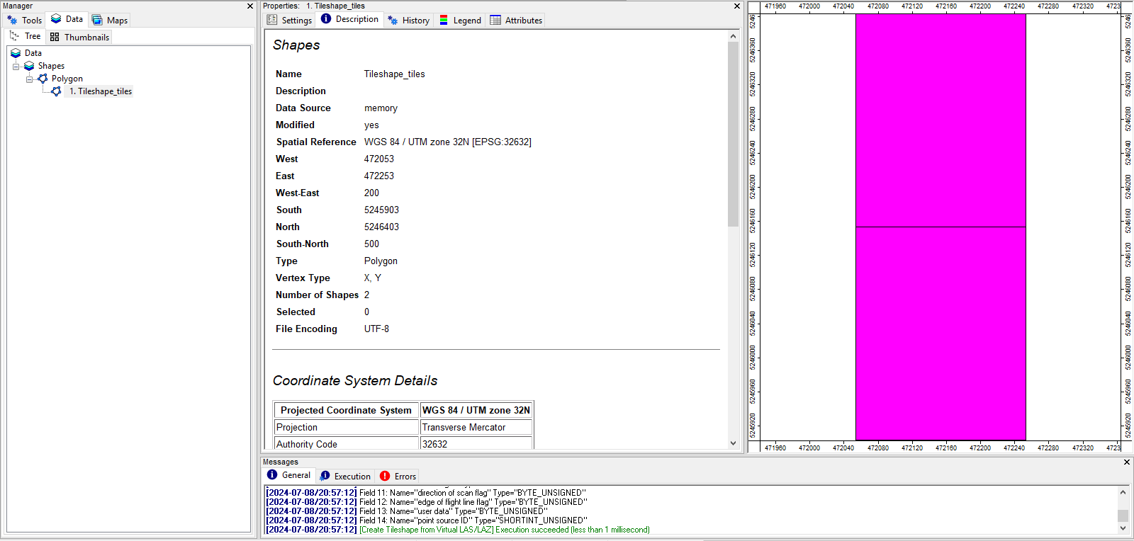
You can find the resulting vector layer with the bounding boxes in the data tab
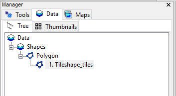
Double-click on it in order to open it in a map.
You can see the bounding box of both laz-files as shapefiles.
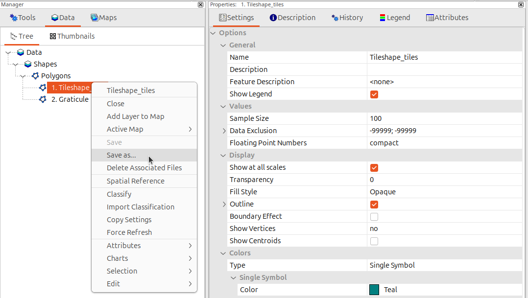
Save this vector layer into the shapes folder of your project (right click on Tileshape_tiles, then Save as):
Create Tiling Scheme for Processing the Data
Create a new tiling scheme for processing the data by running Create Spatial Processing Units. This can be absolutely independent from the bounding boxes (i.e., the physical tiling) of your input data which we generated in the previous step.
- Provide Tileshape_tiles as Extent
- Choose Rectangles in order to get a polygon output
- Choose Round
- Choose Division Height and Division Width, use 100m
- Click Execute
Tool: Create Spatial Processing Units
Geoprocessing → LIS Pro 3D → Tools → Shapes // Tools → LIS Pro 3D → Tools
| Parameter | Setting |
|---|---|
| Data Objects | |
| Shapes | |
| << Units | <create> |
| Options | |
| Extent and Tile Size | |
| > Extent | 1. Tileshape_tiles |
| Tile Size | 100 |
| Adaptive Subdivision | |
| Subdivision | none |
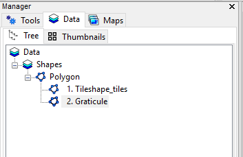
The processing units appear in the data tab
Double-click on it, in order to add it to the existing map.
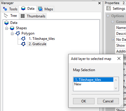
In the Maps Tab toggle between both datasets of the map by clicking on them.
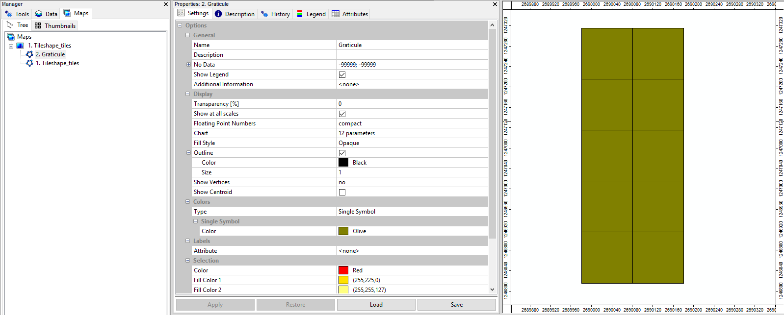
You can see that you have created a much smaller tiling scheme of processing units compared to the extent of the input files. Click “Save as” and save this vector layer as Tiles_100.shp.
Create Additional Tiling Schemes
These will be used later for slicing the dataset after processing.
Create Tiling Schemes with Tile Size 300
Now repeat the previous step and create a tiling scheme with a grid size of 300 m. Save this 300 m tiling scheme into the shapes folder of your project as Tiles_300.shp.
Create Tiling Scheme with One Single Tile
Use Shapes > Tools > Get Shapes Extents and give it the 100 m grid as input with the following options:
Tool: Get Shapes Extents
Geoprocessing → Shapes → Tools // Tools → Shapes → Tools
| Parameter | Setting |
|---|---|
| Data Objects | |
| Shapes | |
| >> Shapes | Tiles_100 |
| << Extents | Extents |
| Options | |
| Get Extent for … | all shapes |
Save the resulting vector layer with the extent in the shapes folder of your project as single_tile_graticule.shp!
Recap
We have designed a data preparation workflow in the GUI. Thereby, we have added las-index files (.lax) to the data/las folder and created a virtual point cloud file (*.lasvf).
Furthermore we have added different tile shapes (*.shp ) to the processing/shapes folder:
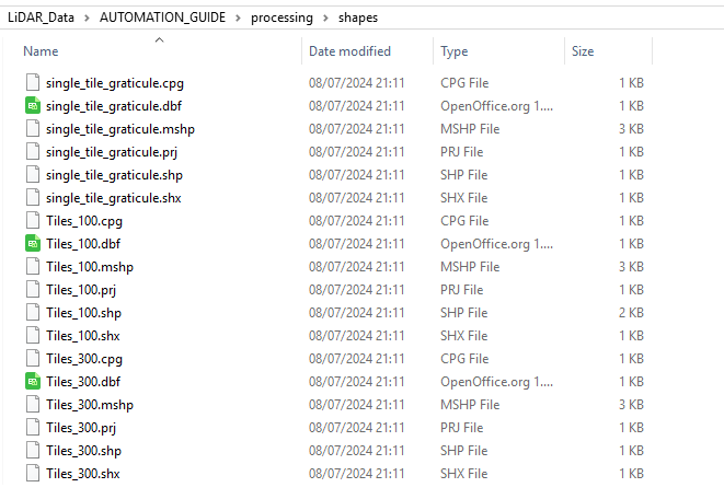
The workflow includes the preparation of folders and these four main steps:
- Create LAS/LAZ index
- Create a point cloud catalog
- Create a vector dataset containing the extent of each of the input files
- Create a tiling scheme for processing with a specified grid spacing (e.g., 100 m and 300 m)