Overview and Visualization of Data for Classification Tutorial
Overview
In this tutorial you will learn how to turn a raw, unclassified point cloud into a fully classified point cloud. In the end, the point cloud will be classified into ground, low, medium and high vegetation, buildings, powerlines and pylons. All of this functionality is available with the basic LIS Pro 3D installation, i.e., does not require any of the LIS Pro 3D addons!
In the following, you will use the LIS Pro 3D graphical user interface for inspecting the test dataset:
Step 0: Download Data for This Tutorial
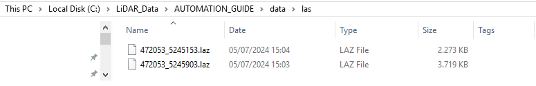
Here you can find two laz-files, which we will use throughout this tutorial. This data is available from the Canton of Zurich under the CC-BY-4.0 license.
Download these two files:
472053_5245153.laz472053_5245903.laz
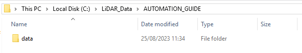
Step 1: Create Folder Structure for Your Project
First, create a top-level directory for the project. Here, this is called AUTOMATION_GUIDE.
Create a Folder for Your Input Data
Create a folder called data with the subfolder las and put your available input *.laz-files in it! Please note, that you don’t necessarily need to perform this step if you already have a dataset somewhere else on your PC.
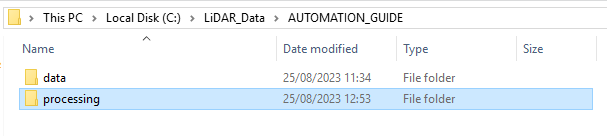
Create a Processing Folder
Here, we will save all the output files that we produce during processing:
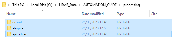
Create Your Output Folders
Within the processing folder, create the folders, where all the actual outputs will be saved! These folders are called:
- export (the folder for your final output)
- shapes (the folder for shapefiles describing the extent of your available data)
- spc_class (the folder for the classified output pointclouds)
Step 2: Import the Available LAZ Files
First, open LIS Pro 3D!
We have two *.laz-files available that we can import and inspect:
- 472053_5245903.laz
- 472053_5245153.laz
Let’s import the two *.laz-files using the tool Import LAS/LAZ Files.
In all our tutorials, we describe the execution of individual tools via the Tool Libraries interface. If you are not familiar with executing tools this way, please consult this section in our introductory tutorial series. In this section, we describe how you can locate the tools in LIS Pro 3D’s GUI.
Tool: Import LAS/LAZ Files
Geoprocessing: LIS Pro 3D → Import/Export → LAS/LAZ // Tools → LIS Pro 3D → LAS/LAZ Files
| Parameter | Setting |
|---|---|
| Input Files | “C:\…path to…\472053_5245903.laz” |
| Attributes to import besides x,y,z … | |
| GPS-time | ☐ |
| Number of the return | ☐ |
| Number of returns of given pulse | ☐ |
| Intensity | 🗹 |
| Classification | ☐ |
| Classification flags | ☐ |
| Synthetic flag | ☐ |
| Keypoint flag | ☐ |
| Withheld flag | ☐ |
| Overlap flag | ☐ |
| Red channel color | ☐ |
| Green channel color | ☐ |
| Blue channel color | ☐ |
| RGB color | ☐ |
| Near infrared | ☐ |
| Scan angle | ☐ |
| Direction of scan flag | ☐ |
| Edge of flight line flag | ☐ |
| User data | ☐ |
| Point source ID | ☐ |
| Scanner channel | ☐ |
| Extra bytes | ☐ |
| Options | |
| Classes | |
| Last Returns | ☐ |
| R,G,B Value Range | 16 bit |
| Import AOI | ☐ |
| Point Cloud Thinning | ☐ |
- Use the browse button in order to find the Input files in your directory structure
- Choose some attributes (e.g. intensity, as indicated here) in order to add it as an additional attribute field (besides x,y,z) to the point cloud
- Click Execute
Please note that we deliberately do not check the box for importing the classification, which is already present in the laz-file - in this tutorial you will learn how to classify a point cloud from scratch with LIS Pro 3D!
For las/laz-files or sg-pts-z files you can also just drag-and-drop them into the GUI. However, this offers no options to customize the import, such as ignoring the classification attribute.
Step 3: Inspect the Available LAZ Files
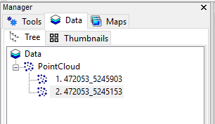
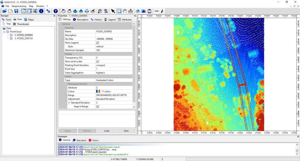
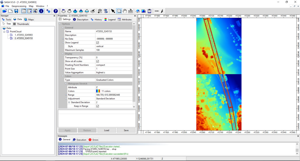
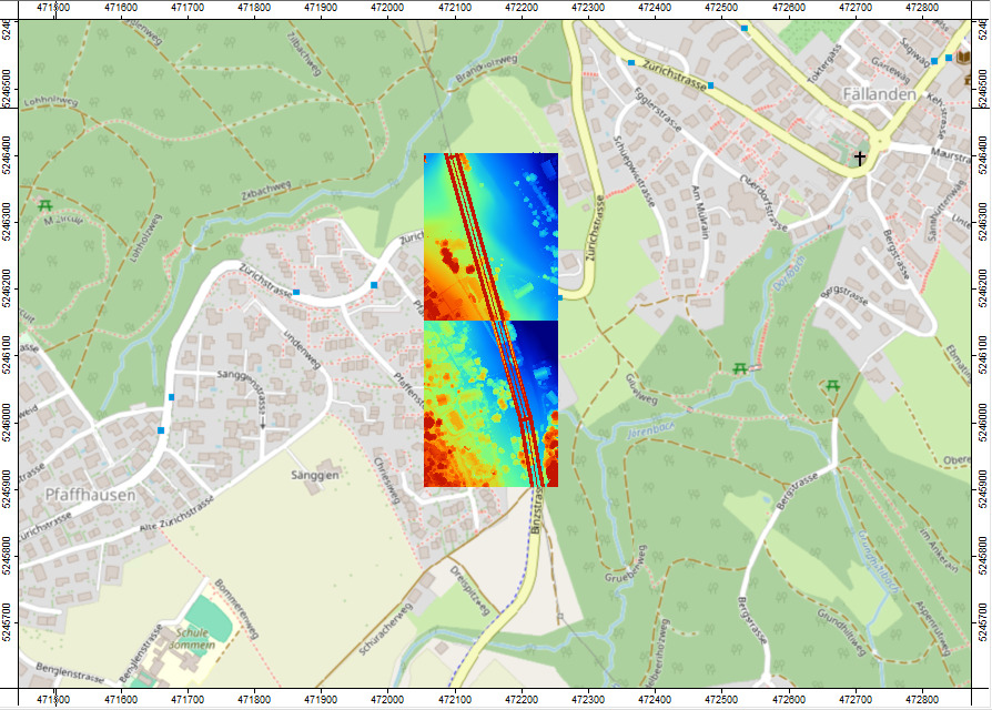
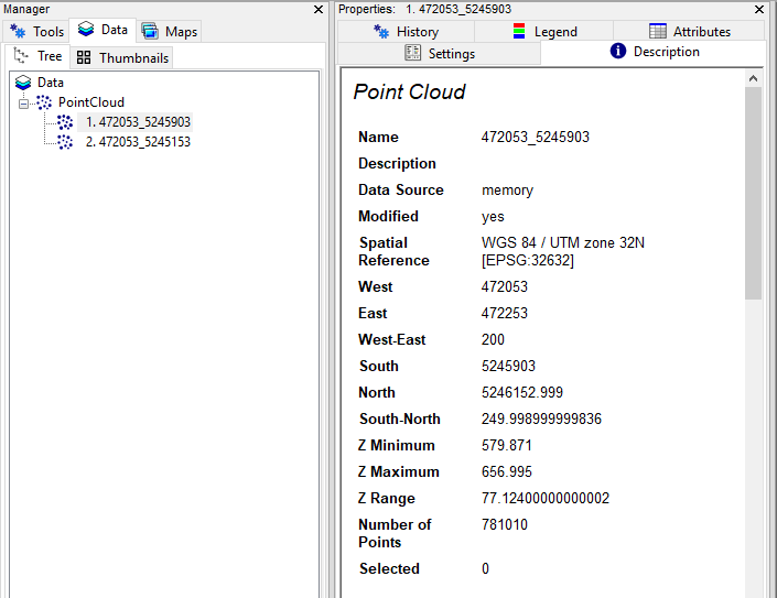
The imported files will appear in the Data Tab of the Manager Window.
Double-clicking onto one of the datasets will open a map-view of the point cloud.
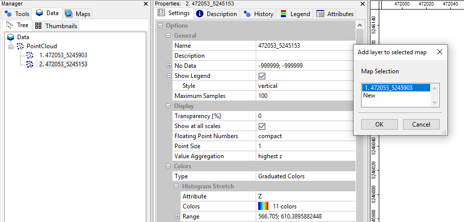
Double-click onto the second dataset and (in the following popup) add it to the existing map (selected in blue here)
Use the Zoom tool (highlighted in blue) in order zoom out in the map.
- Zoom: Mouse Wheel (roll)
- Move: Mouse Wheel (hold and move)
You can see, that we have two separated datasets. We can switch off and on the datasets in the Maps Tab of the Manager Window by clicking on it.
Step 4: Set the Projection of the Dataset
In case you have imported the laz-files via drag-and-drop, the pointcloud dataset has not yet a projectionassigned. In this case, we have to define the correct projection first, before viewing the dataset together with a Web Mapping Service (WMS).
It is recommended to always define the correct projection after import, to make sure everything is set correctly
Tool: Set Coordinate Reference System
Geoprocessing → Projection → Tools // Tools → Projection → PROJ
| Parameter | Setting |
|---|---|
| Data Objects | |
| Grids | |
| > Grids | No objects |
| Shapes | |
| > Shapes | 2 objects (472053_5245903, 472053_5245153) |
| Options | |
| Definition String | +proj=utm +zone=32 +datum=WGS84 +units=m +no_defs +type=crs |
| Display Definition as… | PROJ |
| Authority Code | 32632 |
| Authority | EPSG |
| Well Known Text File | |
| Geographic Coordinate Systems | <select> |
| Projected Coordinate Systems | <select> |
| Pick from Data Set | |
| Data Objects | |
| Grids | |
| Grid system | <not set> |
| > Grid | <not set> |
| Shapes | |
| > Shapes | <not set> |
| Customize | |
| Options | |
| Projection Type | Universal Transverse Mercator (UTM) |
| Datum Definition | Predefined Datum |
| General Settings | |
| Projection Settings | |
| Zone | 32 |
| South | ☐ |
| Predefined Datum | WGS84 |
| Unit | Meter (1) |
| Ignore Defaults | 🗹 |
- Pass the two laz-files in the
> Shapessection - Set the
Authority Codeto32632(UTM32N) - All other parameters will update automatically
- Click Execute
Step 5: Add a Basemap
We can now add a basemap to our mapview in order to see where our data is located.
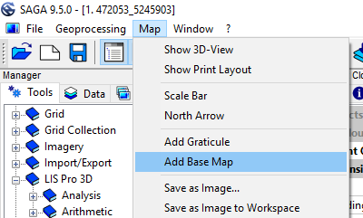
In the top menu you can click on Map > Add BaseMap and choose a layer as basemap (e.g. Open Street Map).
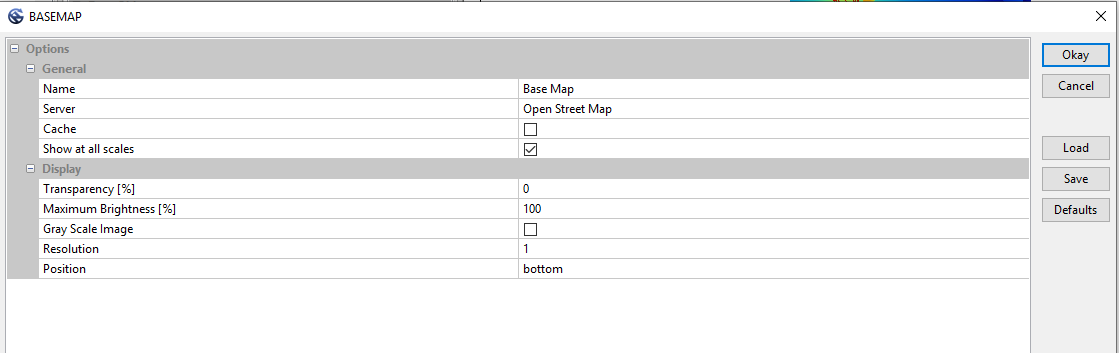
click okay!
In the Mapview a new background layer appears.
This is only working if the loaded layers have a correct projection assigned (e.g., UTM 32N in the example given here). The assigned projection can be reviewed by selecting the respective dataset and inspect the Spatial Reference in the Description Tab.
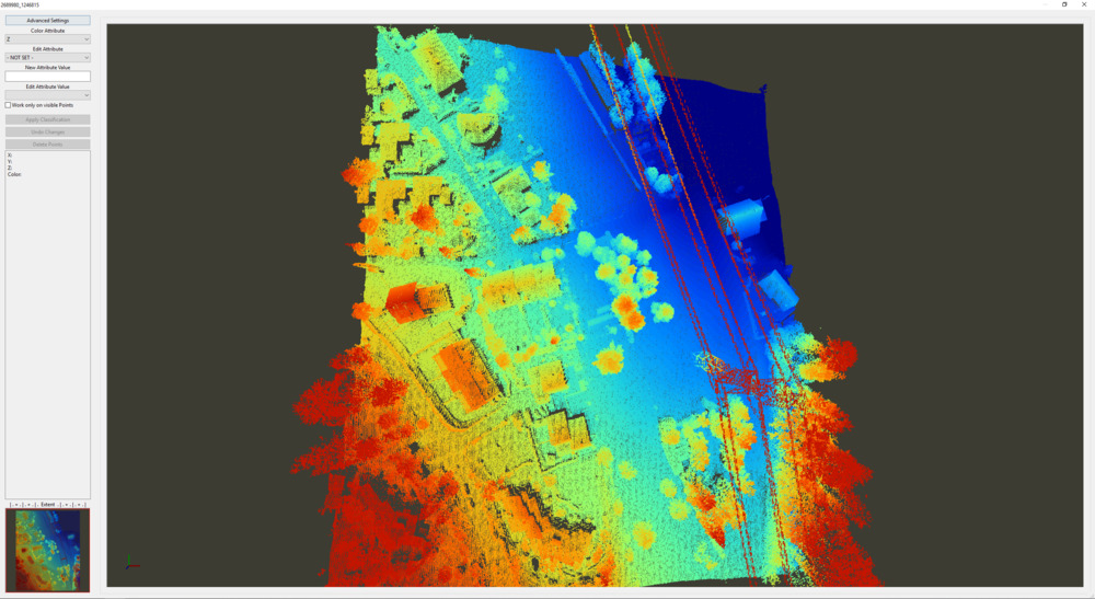
Step 6: Inspect the Available LAZ Files in 3D
Use the tool Point Cloud Editor in order to view a dataset in 3D.
Tool: Point Cloud Editor
Geoprocessing: LIS Pro 3D → Point Cloud Editor // Tools → LIS Pro 3D → Point Cloud Editor
| Parameter | Setting |
|---|---|
| >> Point Cloud | 472053_5245903 |
| Intensity | intensity |
| RGB | <not set> |
| Shading | <not set> |
| Classification | <not set> |
| Random | <not set> |
| Normal Vector (X) | <not set> |
| Report Attribute 1 | <not set> |
| Report Attribute 2 | <not set> |
| Grids | |
| > Elevation Grids | No objects |
| > Color Grids | No objects |
| Shapes | |
| > Shapes | <not set> |
| Options | |
| Work on Copy of Point Cloud | ☐ |
| Background Color | Black |
- Provide a point cloud (here named 472053_5245903) and the intensity attribute
- Click Execute
The Point Cloud Editor opens. The following are the most important operations and keyboard shortcuts to remember when working with the LIS Pro 3D Point Cloud Editor:
- rotate the point cloud with hold/drag left mouse
- move the point cloud with hold/drag right mouse
- zoom the point cloud with mouse wheel
- select a subsection in the lower left window by dragging a rectangle with left mouse
- select a profile in the lower left window by dragging a line with right mouse
- switch to intensity coloring by typing the shortcut 2 on your keyboard.
- increase/decrease the point size by typing the shortcut F6/F5 on your keyboard.
- change transparency of points by typing the shortcut F12/F11 on your keyboard.
Close the Point Cloud Editor again by clicking on the x in the up-right corner of your screen.