SAGA & LIS Pro 3D Quickstart
What You Find in This Section
This section contains a few topics that help you to quickly get started with SAGA and LIS Pro 3D.
- How to import, process and save a raster dataset
- How to import, process and save a point cloud
- How to add a base map
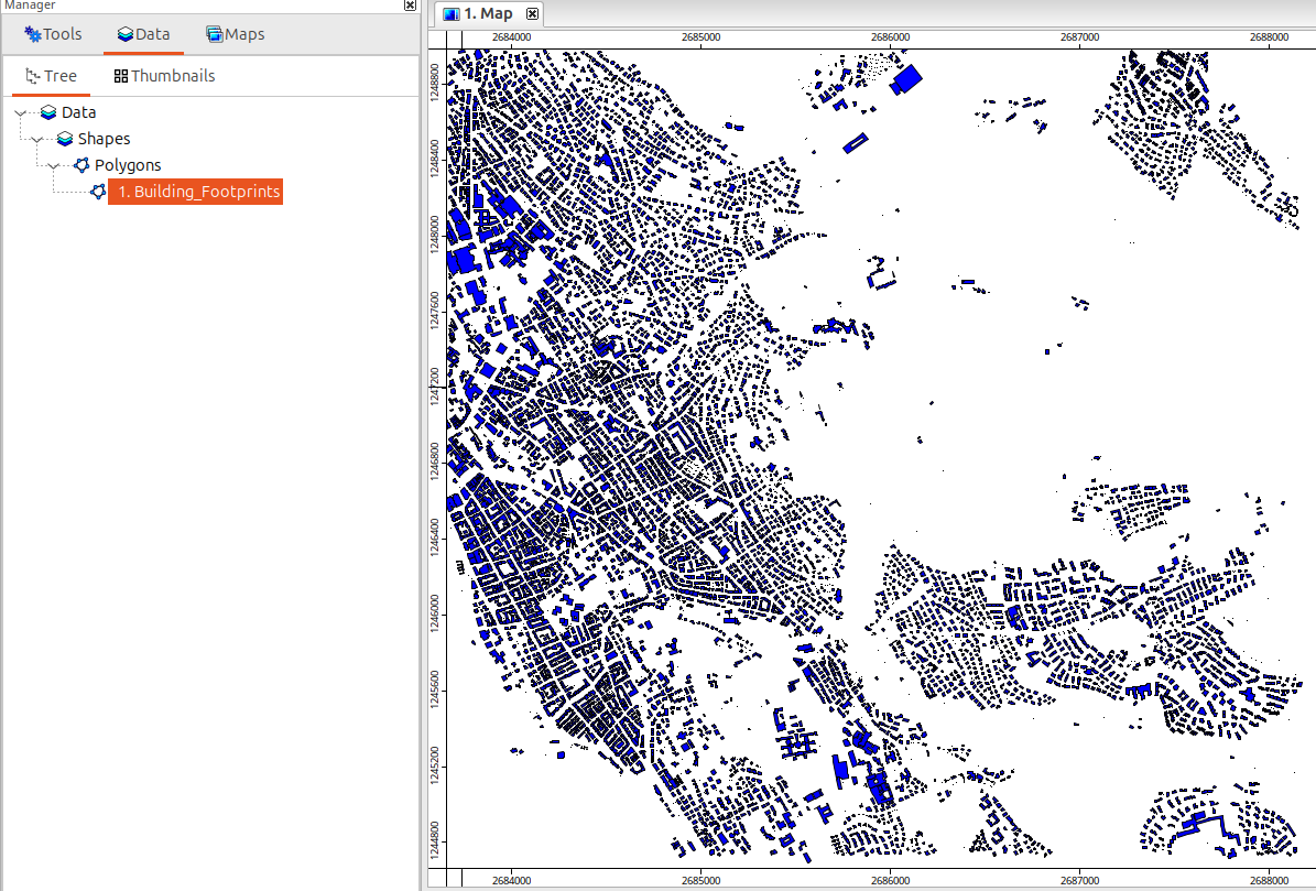
You can follow the import-process-save examples with this dataset which is provided as open data by the Canton of Zurich. This dataset is comprised of a point cloud (.laz file), a digital surface model (.tif file) and a polygon shapes layer with building footprints (.zip file).
How to Import, Process and Save a Raster Dataset
Import
All GDAL-supported file formats can be imported via Import Raster:
In all our tutorials, we describe the execution of individual tools via the Tools interface. If you are not familiar with executing tools this way, please consult this section in our introductory tutorial series. In this section, we describe how you can locate the tools in LIS Pro 3D’s GUI.
Tool: Import Raster
Geoprocessing → File → Grid // Tools → Import/Export → GDAL/OGR
| Parameter | Setting |
|---|---|
| Options | |
| Input | Files |
| Files | “/path/to/…./2684500_1247000.tif” |
| Multiple Bands Output | automatic |
| Select from Multiple Bands | ☐ |
| Transformation | 🗹 |
| Resampling | Nearest Neighbour |
| Extent | original |
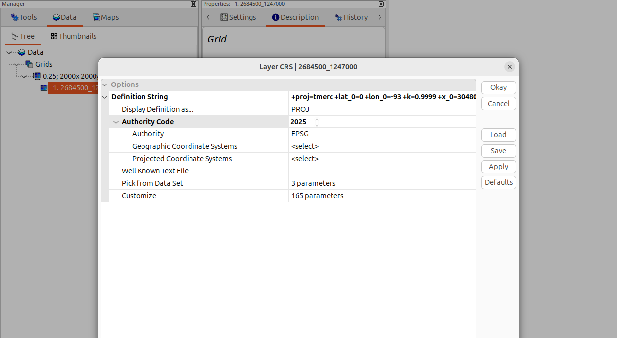
We recommend to always explcitly assign the projection. If the projections settings are incorrect or incomplete, files may be misaligned. Right-click onto the file:
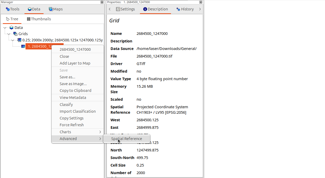
Delete and type the Authority Code 2056 again into the respective field. Confirm by pressing ENTER. The field should indicate with bold letters that is has been updated. Click Okay to finish:
Note: many raster file formats can also be imported via drag-and-drop to the GUI.
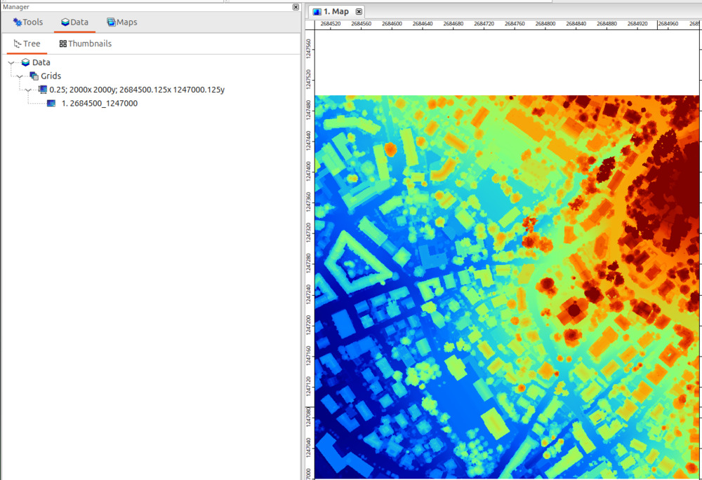
Perform a double-click on the dataset in the “Data” tab of the “Manager” window to add it to a map.
Process
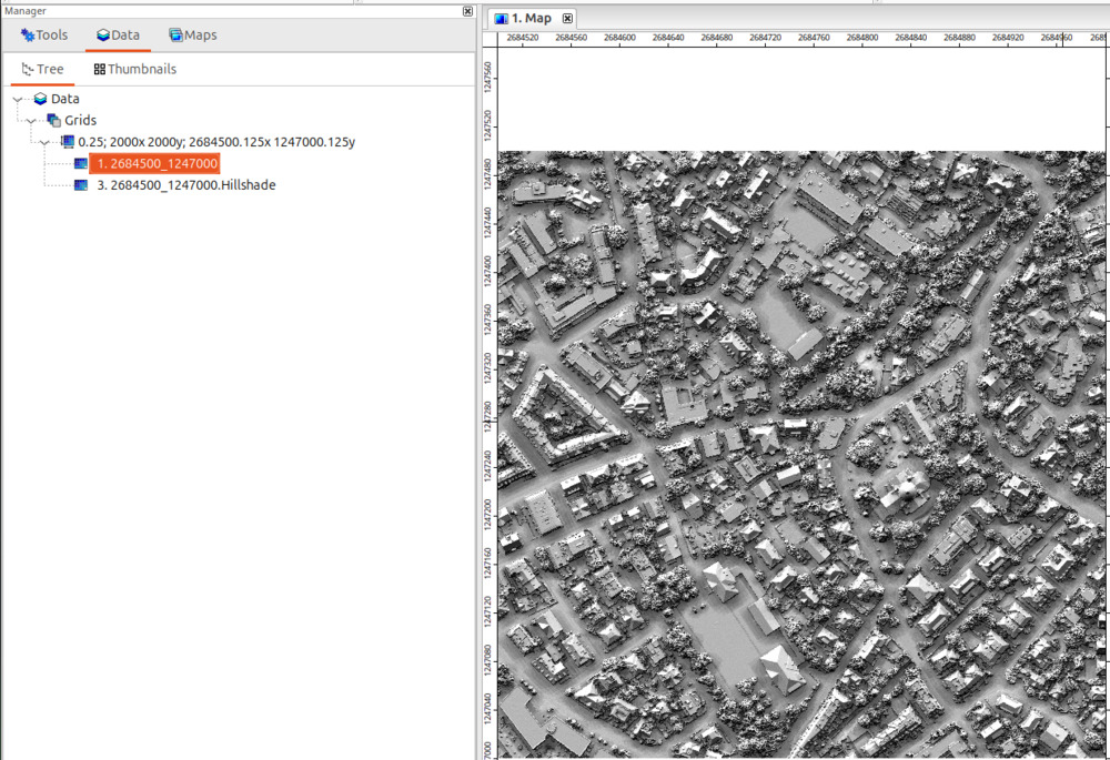
As processing example, we will create a shading from the digital surface model:
Tool: Analytical Hillshading
Geoprocessing → Terrain Analysis → Lighting and Visibility // Tools → Terrain Analysis → Lighting & Visibility
| Parameter | Setting |
|---|---|
| Data Objects | |
| Grids | |
| Grid System | 0.25; 2000x, 2000y; 2684500…x 1247000…y |
| >> Elevation | 2684500_1247000 |
| << Analytical Hillshading | <create> |
| Options | |
| Shading Method | Ambient Occlusion |
| Sampling Hemisphere | north |
| Number of Directions | 8 |
| Search Radius | 10 |
Save or Export
SAGA holds all its datasets in memory during processing. Therefore you explicitly need to save the processing results to disk in order to store them permanently.
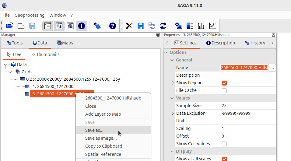
Do a right-click on the dataset in the “Data” tab of the “Manager” window and choose “Save as…” from the context menu. The file dialog allows to store the raster in SAGA’s native grid format (*.sg-grd or compressed *.sg-grd-z) or as GeoTIFF (*.tif). For other GDAL-supported file formats, use the Export Raster tool.
How to Import, Process and Save a Point Cloud
Import
Point clouds in SAGA’s native format (*.sg-pts and compressed *.sg-pts-z) can be loaded via drag-and-drop to the GUI. Other file formats (*.rdbx, *rxp, *.las/*.laz, text-files) need to be imported via dedicated tools (Tools → LIS Pro 3D → Import/Export). To load the example “2684500_1247000.laz” file, we use the Import LAS/LAZ Files tool and import only the classification field (besides the x,y,z coordinates):
Tool: Import LAS/LAZ Files
Geoprocessing → LIS Pro 3D → Import/Export → LAS/LAZ // Tools → LIS Pro 3D → Import/Export
| Parameter | Setting |
|---|---|
| Options | |
| Input Files | “/path/to/…/2684500_1247000.laz” |
| Attributes to import besides x,y,z … | |
| Number of returns of given pulse | … |
| … | … |
| Intensity | 🗹 |
| Classification | 🗹 |
| … | … |
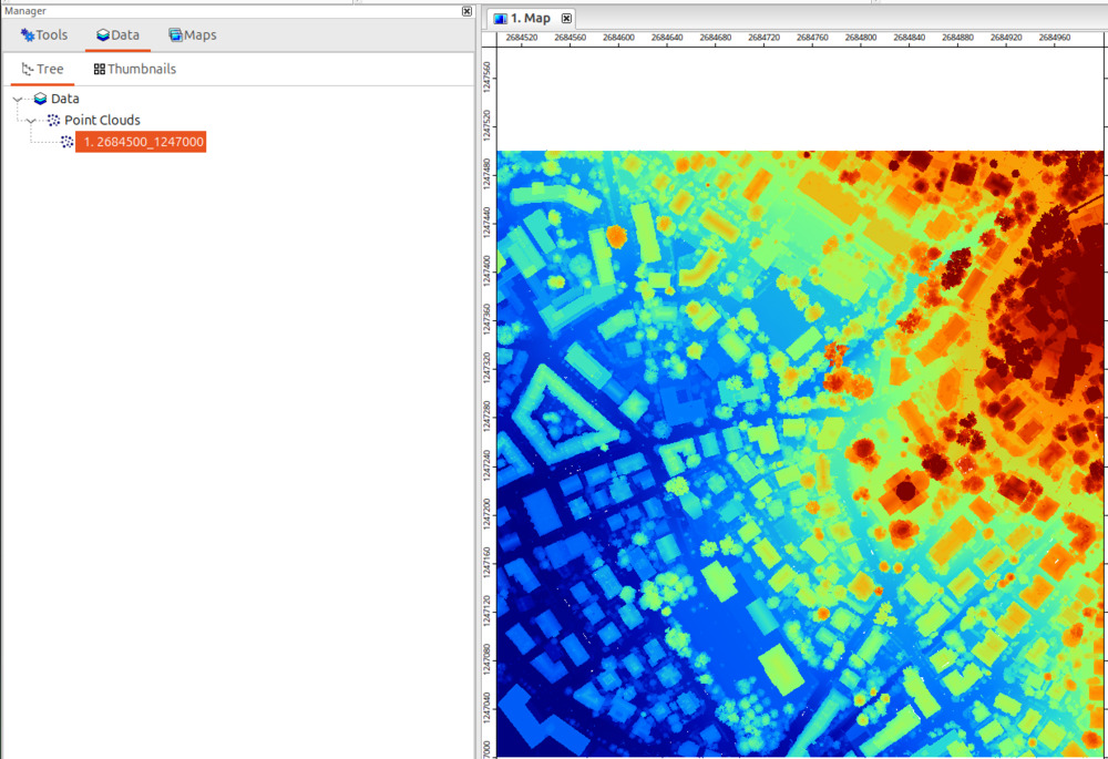
To add the loaded point cloud to the map, do a double-click on the dataset in the “Data” tab of the “Manager” window.
Process
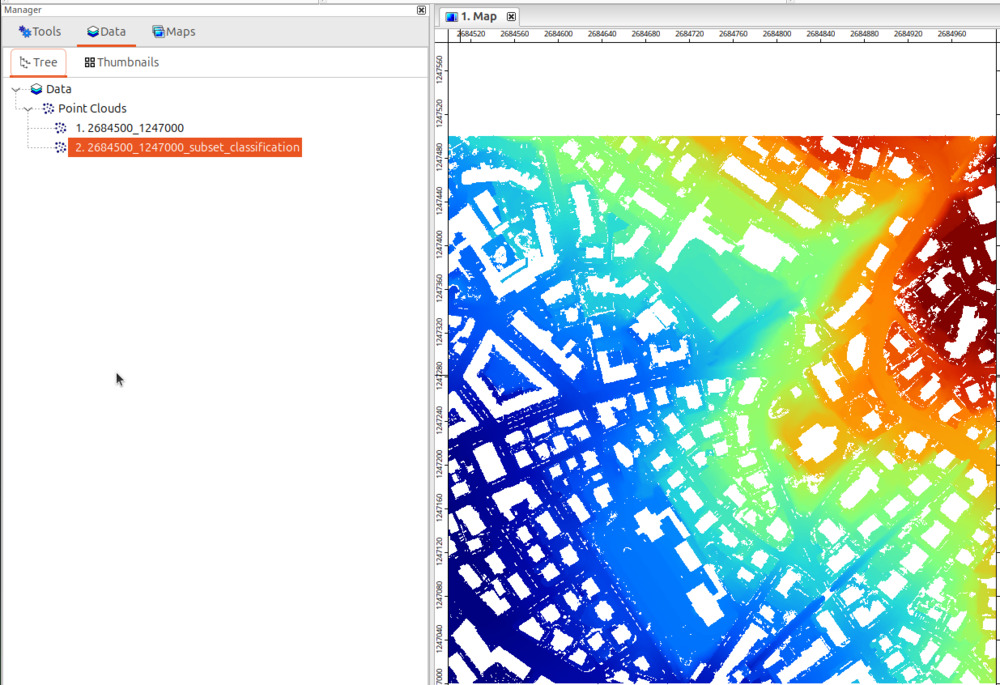
As a processing example, we will extract all points labelled as “ground” (ASPRS LAS class 2) from the dataset:
Tool: Extract Subset from Point Cloud
Geoprocessing → LIS Pro 3D → Tools → Point Cloud → Subsetting // Tools → LIS Pro 3D → Tools
| Parameter | Setting |
|---|---|
| Data Objects | |
| Point Clouds | |
| >> Point Cloud | 2684500_1247000 |
| Attribute | classification |
| << Point Cloud | <create> |
| Options | |
| Method | single value |
| Single Value | 2 |
| Operator | = single value |
Save or Export
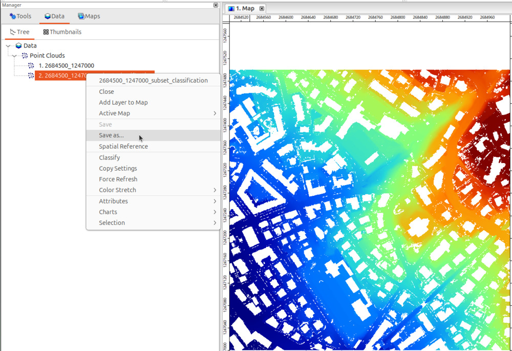
To save the created point cloud permanently to disk in SAGA’s native format (*.sg-pts or compressed *.sg-pts-z), do a right-click on the dataset in the “Data” tab of the “Manager” window and choose “Save as…” from the context menu.
Other file formats (e.g. *.rdbx, *.las/*.laz, or text-files) can be written via dedicated tools (Tools → LIS Pro 3D → Import/Export)!
How to Import, Process and Save Vector Data
Import
ESRI Shapefiles and other GDAL-supported vector file formats can be loaded via drag-and-drop to the GUI or with dedicated tools. Here, we show the usage of the Import Shapes tool to load Building_Footprints.shp file:
Tool: Import Shapes
Geoprocessing → File → Shapes // Tools → Import/Export → GDAL/OGR
| Parameter | Setting |
|---|---|
| Options | |
| Files | “/path/to/…/Building_Footprints.shp” |
The shapes layer can be added to the map by double clicking it in the “Data” tab.
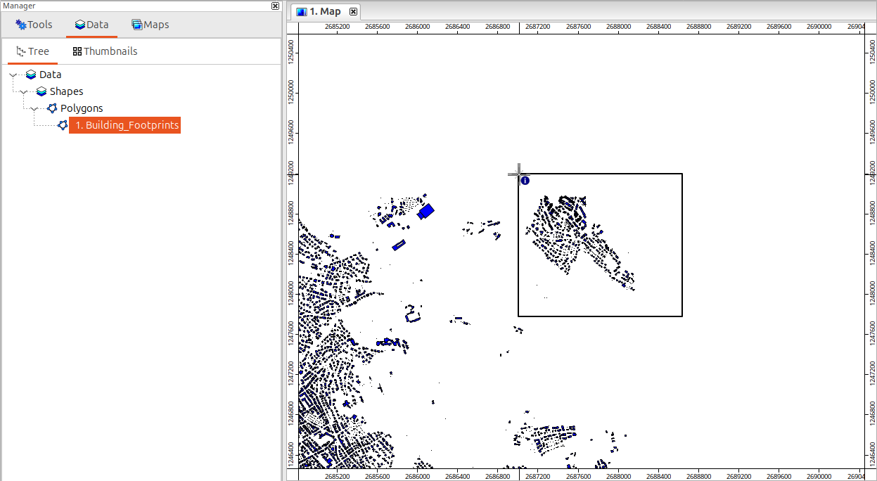
Process
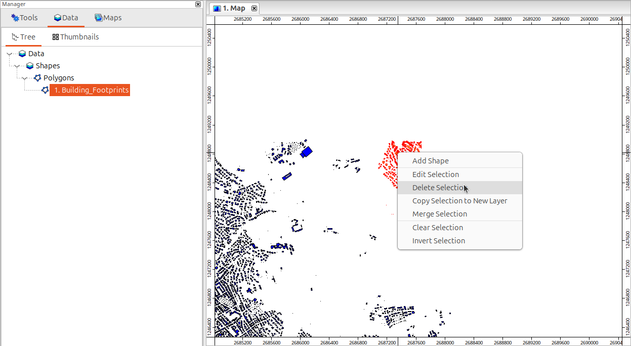
As a processing example, we will simply delete a handful of polygons. Pan and zoom to the upper right corner and select (selection is possible by dragging a polygon on the map when the interact cursor is active) a handful of buildings:
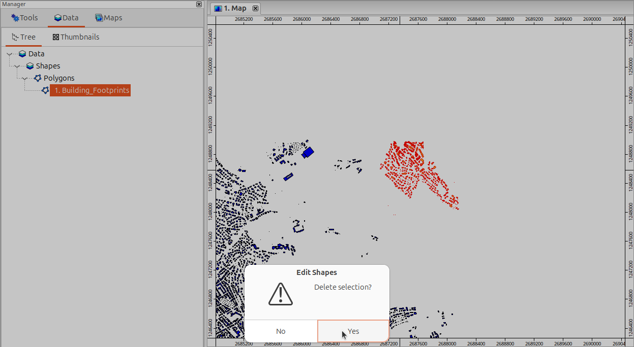
Rigth-click to remove the buildings:
Confirm:
Save or Export
To save any shapes layer permanently to disk, do a right-click on the dataset in the “Data” tab of the “Manager” window and choose “Save as…” from the context menu:
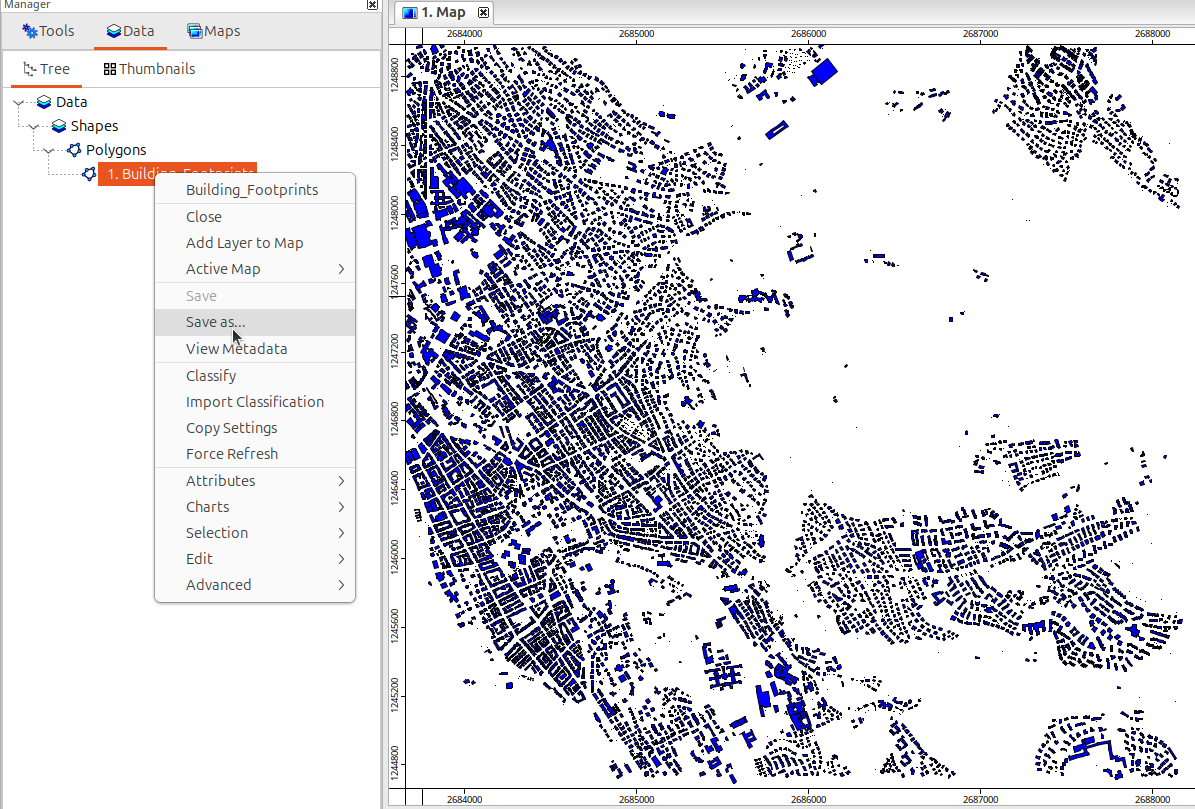
Note that the file dialog only allows you to save the dataset in ESRI Shapefile, GeoJSON or GeoPackage format. Other file formats can be written with the Tools > Import/Export > GDAL/OGR > Export Shapes tool.
Maps
How to Add a Base Layer to the Map
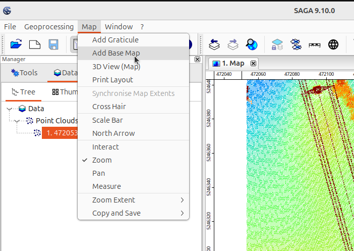
It is possible to add a base map to an existing map. Once a map view is open, the “Map” menu will be available (see Figure 1).
If your map does not have a valid spatial reference system defined, the “Add Base Map” menu entry will be greyed out. This happens when the first dataset added to the map had no spatial reference assigned. To define the spatial reference used by the map, right-click on the map in the “Maps” tab of the “Manager” window and choose “Spatial Reference” from the context menu. In the dialog that opens, you can set the spatial reference system in various ways, e.g. by providing an EPSG code.
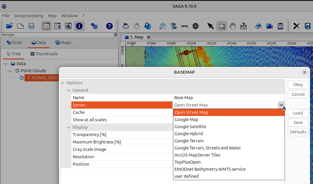
Once the base map dialog opens, you can choose among different base map providers. Click “Okay” to add the desired base map.
Pan/Zoom to a Dataset in a Map
Do a right-click on the respective data object in the “Data” tab of the “Manager” window and select the desired option:
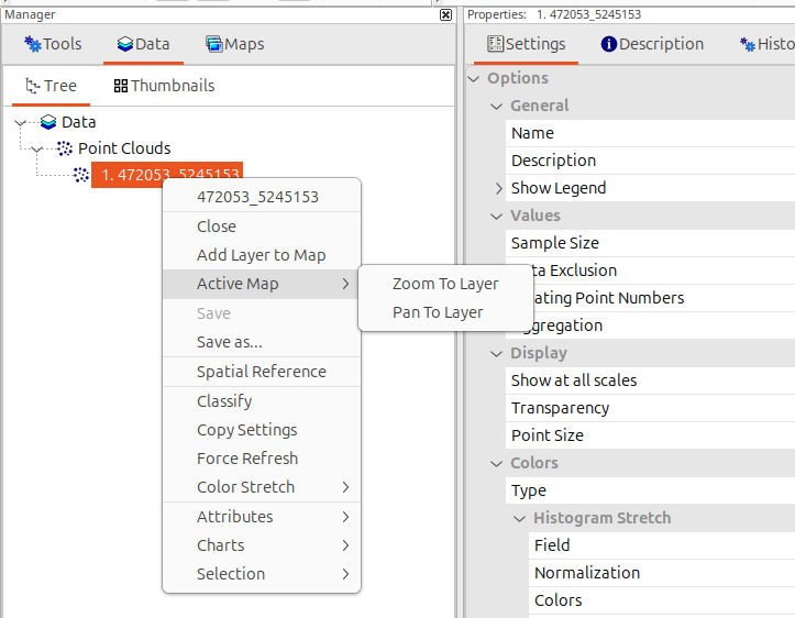
The same options are available when you do a right-click on a map layer in the “Maps” tab of the “Manager” window.
3D Point Cloud Visualization
To view the point cloud in 3D, we use the Tools → LIS Pro 3D → Point Cloud Editor tool. Provide the point cloud and set the classification and intensity attributes (which allows us to use shortcuts for coloring):
Tool: Point Cloud Editor
Geoprocessing → LIS Pro 3D → Point Cloud Editor // Tools → LIS Pro 3D → Point Cloud Editor
| Parameter | Setting |
|---|---|
| Data Objects | |
| Point Clouds | |
| >> Point Cloud | 2684500_1247000 |
| Intensity | intensity |
| RGB | <not set> |
| Shading | <not set> |
| Classification | classification |
| Random | <not set> |
| Normal Vector (X) | <not set> |
| Report Attribute 1 | <not set> |
| Report Attribute 2 | <not set> |
| Grids | |
| > Elevation Grids | No objects |
| > Color Grids | No objects |
| Shapes | |
| > Shapes | <not set> |
| Options | |
| Work on Copy of Point Cloud | ☐ |
| Background Color | #3C3C32 |
| Classification LUT | ASPRS LAS (Formats 6-10) |
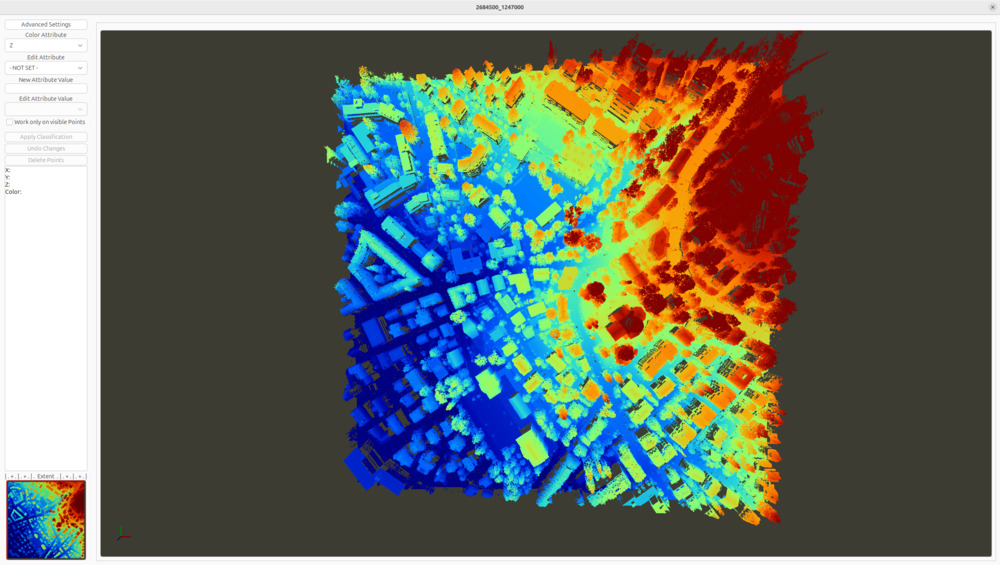
When you execute the tool, a window will open and display the point cloud colored by elevation:
Please note: depending on the number of points and the resources of your computer, this may take a moment. You can use the scroll wheel of the mouse for zooming. Right-click + dragging will move the point cloud left/right/top/bottom.
Here is a list of some frequently used keyboard shortcuts which allow you to change the visualization settings in LIS Pro 3D’s Point Cloud Editor:
- r: reset view to default extent and viewing direction
- 1: color point cloud by elevation
- 2: color point cloud by intensity
- 5: color point cloud by classification
- q: color randomly by the field given as “Random” - this is handy, for example, to visualize the output of a point cloud segmentation
- F5/F6: de-/increase point size
- F11/F12: de-/increase point cloud transparency
- p: toggle parallel and central projection
The full list of keyboard shortcuts can be found the Description tab of the tool. Please note that coloring by intensity, classification and other attributes requires setting these fields in the tool before opening the point cloud editor.
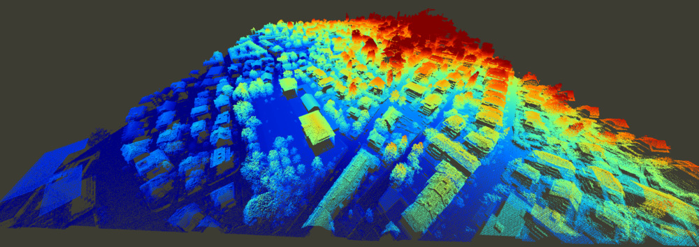
Colored by elevation (the default)
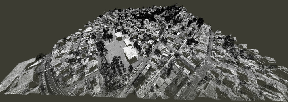
Colored by intensity
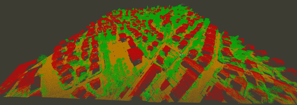
Colored by classification