Structural Geology - Data Processing
< Previous section Next section >
Normal Vectors
Surface normal vectors describe the local orientation of a surface and are calculated for each point in the point cloud. Since the objective is to characterize planar discontinuity surfaces, it is essential to preserve sharp edges and boundaries between individual discontinuities. This requires a robust normal estimation algorithm; otherwise, normal vectors may become distorted across discontinuity boundaries, reducing the accuracy of orientation measurements.
For vertical and overhanging sections of the rock face, it is not mathematically possible to determine whether a computed normal vector points into the rock mass or outward, where it should ideally point. This is where the previously computed “direction-to-scanner” attribute becomes essential.
Tool: Normal Estimation (Robust PCA)
Geoprocessing → LIS Pro 3D → Analysis // Tools → LIS Pro 3D → Analysis
| Parameter | Setting |
|---|---|
| Data Objects | |
| Point Clouds | |
| >> Point Cloud | rock_face |
| Direction Scanner (X) | dirscan_x |
| Direction Scanner (Y) | dirscan_y |
| Direction Scanner (Z) | dirscan_z |
| < Point Cloud Normals | <not set> |
| < Point Cloud Smoothed | <not set> |
| Options | |
| Copy existing attributes | 🗹 |
| Attribute Suffix | |
| NN Search | |
| Method NN | k nearest neighbors |
| k Nearest Neighbors | 12 |
| Maximum Distance Threshold | 🗹 |
| Maximum Distance | 2 |
| Minimum Number of Neighbors | 5 |
| Normal Estimation | |
| Estimated Noise | 0.01 |
| Minimum Curvature Radius | 0.3 |
The tool attaches three new attributes to the point cloud, corresponding to the x-, y-, and z-components of the normal vector. We can again inspect the result in 3D. To render the point cloud with shading based on the normals, set the “Normal Vector (X)” parameter to the x-component of the normal vector.
Tool: Point Cloud Editor
Geoprocessing → LIS Pro 3D → Point Cloud Editor // Tools → LIS Pro 3D → Point Cloud Editor
| Parameter | Setting |
|---|---|
| Data Objects | |
| Point Clouds | |
| >> Point Cloud | rock_face |
| Intensity | intensity |
| RGB | rgb color |
| Shading | <not set> |
| Classification | <not set> |
| Random | ID |
| Normal Vector (X) | normal_x |
| Report Attribute 1 | <not set> |
| Report Attribute 2 | <not set> |
| Grids | |
| > Elevation Grids | No objects |
| > Color Grids | No objects |
| Shapes | |
| > Shapes | <not set> |
| Options | |
| Work on Copy of Point Cloud | ☐ |
| Background Color | #3C3C32 |
When the viewer starts, change the “Color Attribute” (top left) from “Z” to the “normal_z” attribute. This visualizes the z-component of the normal vector, which already provides a good impression of the different orientations.
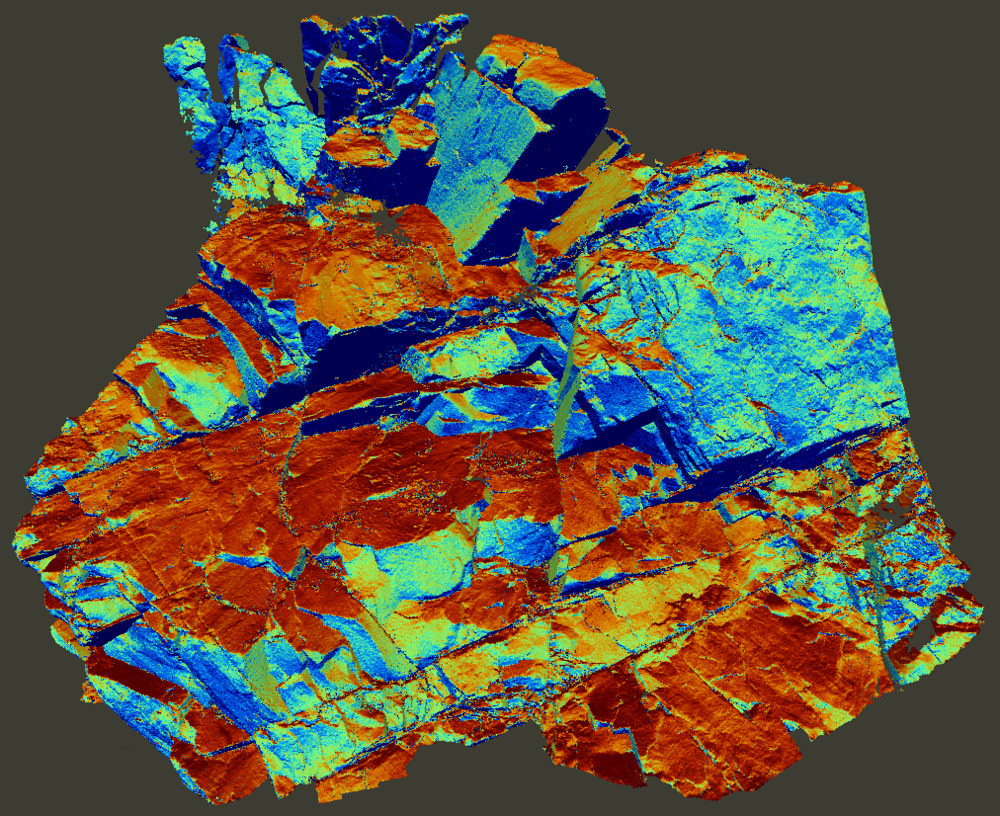 The point cloud colored by the z-component of the derived normal vector.
Identification of Discontinuity Sets
The orientation of discontinuities relative to the overall rock slope geometry provides valuable information for assessing slope stability and identifying potential failure mechanisms. To visualize and analyze the dominant orientations within the rock face, the calculated normal vectors are projected onto a lower-hemisphere pole plot. This stereographic representation displays dip and dip direction of surface elements together with their frequency of occurrence. Because it illustrates the concentration of orientations, it is commonly referred to as a density plot.
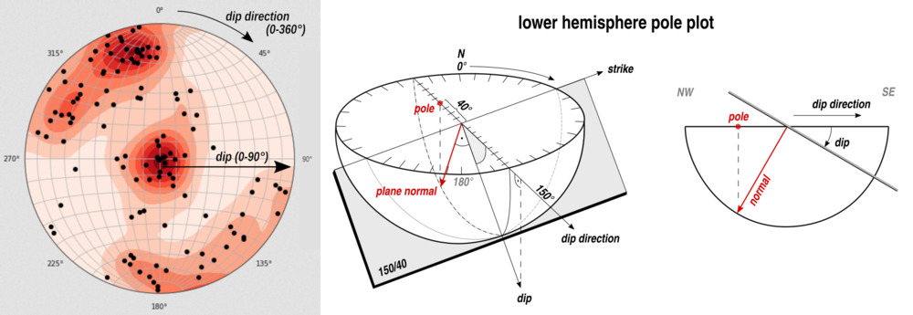 An examplary density plot showing dip direction and dip (left) and an illustration of the lower hemosphere pole plot.
The orientation density distribution shown in the pole plot is used to cluster similar orientations into discontinuity sets, representing the principal joint or fracture systems within the rock mass. Each discontinuity set is characterized by its representative dip and dip direction.
The “Discontinuity Sets” tool creates a pole plot and performs a kernel density estimation to detect local maxima in the plot. These maxima define the poles of potential discontinuity sets. The poles are then filtered (from highest to lowest local maximum) by enforcing a minimum angular separation between them. Subsequently, points are assigned to sets based on a maximum angular difference between each point’s normal vector and the pole of the corresponding set.
Set the “Minimum Normal Difference (Poles)” parameter to 40° and the “Maximum Number of Sets” parameter to 6. Enable all output options.
Tool: Discontinuity Sets
Geoprocessing → LIS Pro 3D → Geology → Point Cloud // Tools → LIS Pro 3D → Geology
| Parameter | Setting |
|---|---|
| Data Objects | |
| Point Clouds | |
| >> Point Cloud | rock_face |
| Normal Vector (X) | normal_x |
| Normal Vector (Y) | normal_y |
| Normal Vector (Z) | normal_z |
| Filter Attribute | <not set> |
| < Point Cloud | <not set> |
| Tables | |
| << Set Information | <create> |
| << Lookup Table | <create> |
| Options | |
| Copy existing Attributes | 🗹 |
| Attribute Suffix | |
| Image of Plot | |
| Radius KDE | 15 |
| Kernel KDE | quartic kernel |
| Minimum Normal Difference Poles | 40 |
| Maximum Number of Sets | 6 |
| Maximum Normal Difference Set | 30 |
| Poles to Suppress | |
| Output | |
| Label Point Cloud | 🗹 |
| Dip Direction and Dip (Set) | 🗹 |
| Dip Direction and Dip (Point) | 🗹 |
| RGB Encoded Orientation | 🗹 |
| Spatial Separation | 🗹 |
| Search Radius | 0.1 |
| Minimum Number of Points | 3 |
| Joint Plane Size | 🗹 |
In practice, the workflow typically starts with an initial tool run without enabling point cloud labelling. This reduces computational time, as only the pole plot is generated as an image output. The parameters can then be adjusted iteratively and the tool re-run until all poles are correctly identified. Once the discontinuity sets are satisfactorily detected, a final run is performed with point cloud labelling enabled, allowing the results to be written back to the point cloud dataset.
The results are output as a rendered image, which is available as a grid in the GUI or can be saved as an image file. Visualize the “plot_rock_face” grid in a map view.
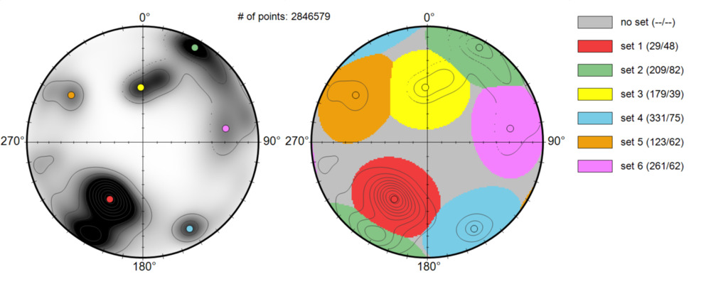 The density plot with poles of the sets (left) and the derived discontinuity sets (right).
The derived discontinuity sets, including their dip direction and dip values, are also reported in a table (“set_info_rock_face”). The tool also creates a lookup table for the sets (“LUT_setid_rock_face”), which can be used for colorization.
The tool creates a set of new point cloud attributes based on the discontinuity sets analysis: - the normal vector of each set (i.e., the normal of the set’s pole) - the dip direction and dip of each set (calculated from the sets’s normal) - the dip direction and dip of each point (calculated from the point’s normal) - dip direction and dip encoded as RGB values (calculated from the point’s normal)
We also activated the “Spatial Separation” parameter in the tool. This option splits the derived sets into individual, spatially separated joint planes by applying a density-based spatial clustering approach within each set. The separation of joint planes is a prerequisite for deriving discontinuity spacing in later steps.
This process creates two additional point cloud attributes: - a unique identifier for each joint plane - the number of points forming each joint plane, which can be used, for example, as a filtering criterion
Let’s take a look at some of the results in the 3D Viewer. Set the “Classification” parameter to the “setid” attribute field and the “Random” parameter to the “jointid” attribute field.
We can also use the generated lookup table to reproduce the same coloring of the sets as used in the pole plot. Set the “Classification LUT” parameter to “User Defined” and provide the “LUT_setid_rock_face” table in the “Lookup Table” parameter.
Tool: Point Cloud Editor
Geoprocessing → LIS Pro 3D → Point Cloud Editor // Tools → LIS Pro 3D → Point Cloud Editor
| Parameter | Setting |
|---|---|
| Data Objects | |
| Point Clouds | |
| >> Point Cloud | rock_face |
| Intensity | intensity |
| RGB | rgb_dipdir |
| Shading | <not set> |
| Classification | setid |
| Random | jointid |
| Normal Vector (X) | normal_x |
| Report Attribute 1 | <not set> |
| Report Attribute 2 | <not set> |
| Grids | |
| > Elevation Grids | No objects |
| > Color Grids | No objects |
| Shapes | |
| > Shapes | <not set> |
| Tables | |
| > Lookup Table | LUT_setid_rock_face |
| Options | |
| Work on Copy of Point Cloud | ☐ |
| Background Color | #3C3C32 |
| Classification LUT | User Defined |
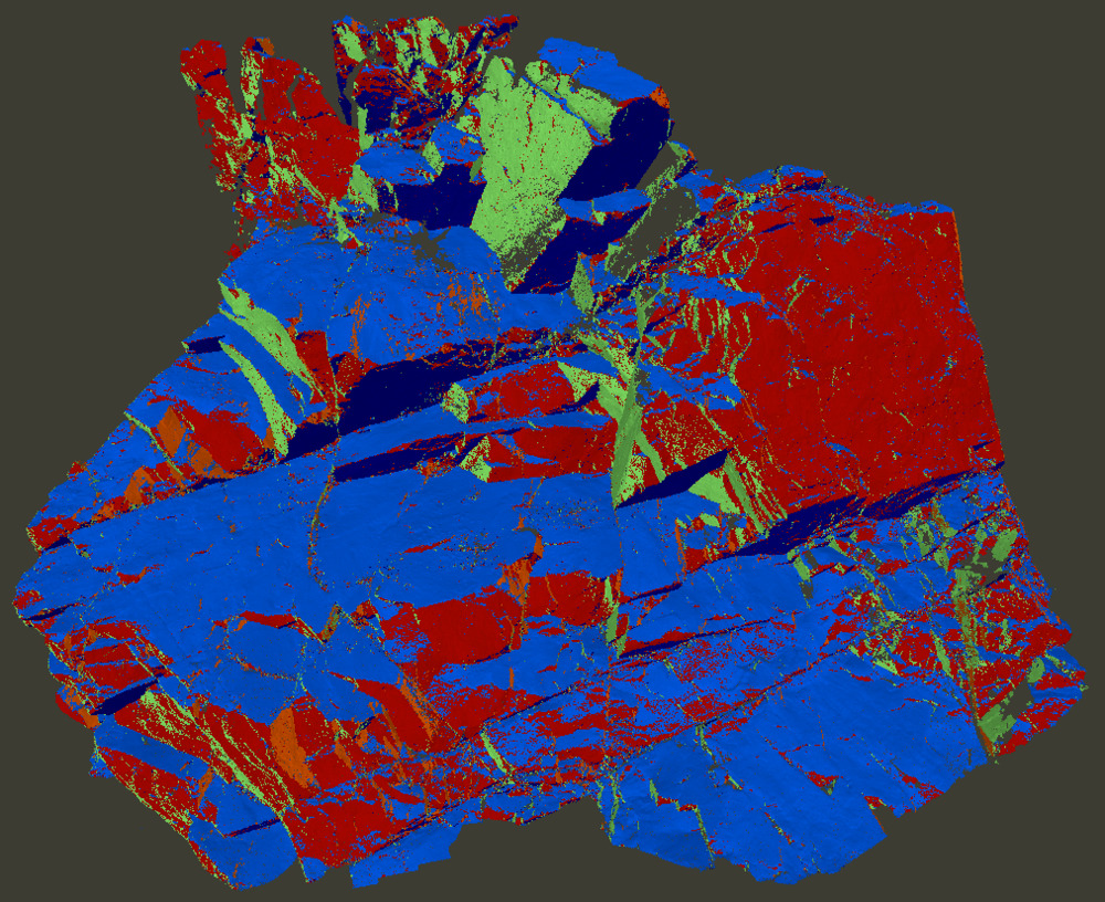
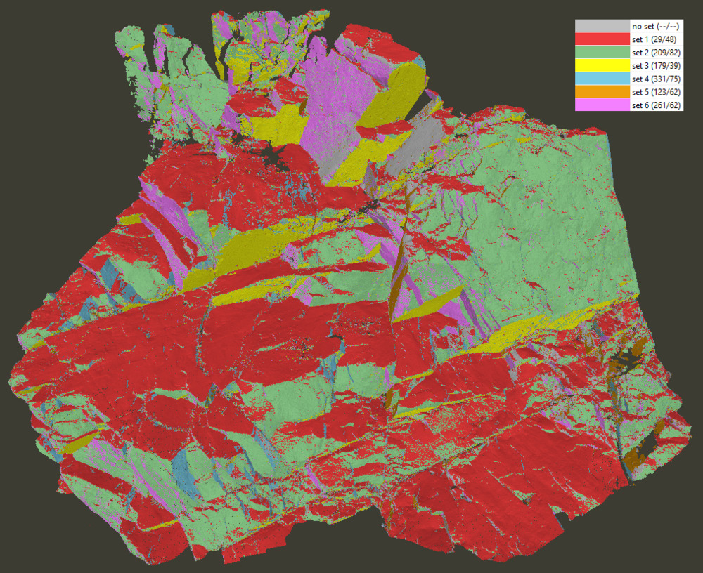 The derived discontinuity sets (keyboard shortcut “5”).
 The dip per set (switch back to elevation coloring using keyboard shortcut “1”; then change the “Color Attribute” from “Z” to the “dip_set” attribute).
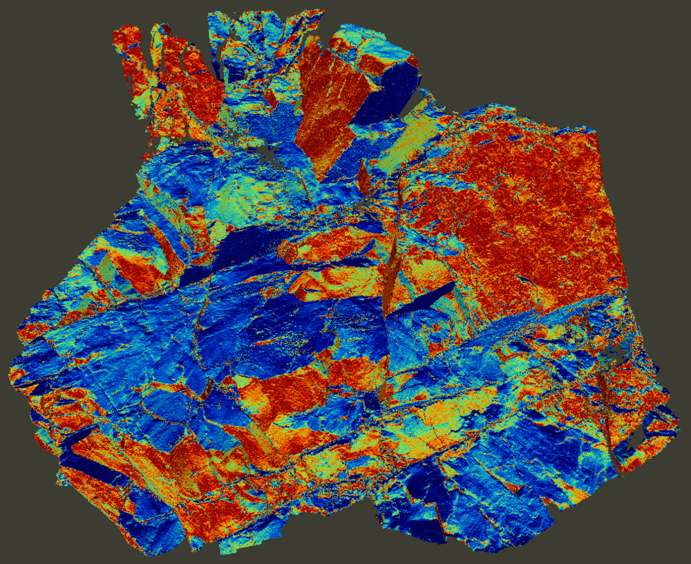 The dip calculated from each point’s normal (set the “Color Attribute” to “dip_pt”).
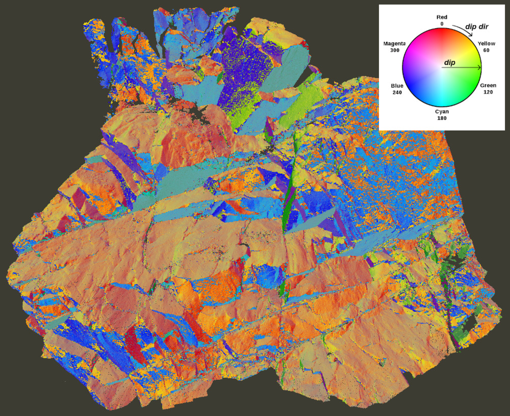 The dip direction and dip encoded as RGB values (keyboard shortcut “3”).
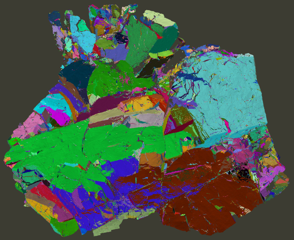 The separated joint planes colored randomly (keyboard shortcut “q”).
If the analysis produces unwanted sets, a list of dip direction and dip values corresponding to the poles to be suppressed can be provided in the “Discontinuity Sets” tool.
Discontinuity Spacing Analysis
Finally, we can analyse the spacing of joint planes within each discontinuity set. Combined with discontinuity orientation, this information can be used to estimate potential block sizes in quarry operations and to support rockfall and natural hazard runout modelling.
The “Discontinuity Spacing” tool computes the non-persistent discontinuity spacing based on the derived set normals and the segmented joint planes. The analysis produces a cumulative frequency distribution of discontinuity spacing for each set, as well as a histogram of spacings. Additional information on set orientation and spacing statistics (number of measurements, mean, standard deviation, and median) is reported in a separate table.
The computation is usually performed on an on-the-fly thinned dataset. This has only minor effects on the results - only the maximum distance used to separate non-persistent discontinuities is influenced - while significantly reducing computational time. Here, we apply a thinning of 30 cm, which affects the “Maximum Distance” of 5 m used to separate non-persistent discontinuities. We also use the “Joint Size” attribute to exclude small joint planes with fewer than 250 points from the analysis.
Tool: Discontinuity Spacing
Geoprocessing → LIS Pro 3D → Geology → Point Cloud // Tools → LIS Pro 3D → Geology
| Parameter | Setting |
|---|---|
| Data Objects | |
| Point Clouds | |
| >> Point Cloud | rock_face |
| Set ID | setid |
| Set Normal Vector (X) | set_normal_x |
| Set Normal Vector (Y) | set_normal_y |
| Set Normal Vector (Z) | set_normal_z |
| Joint ID | jointid |
| Joint Size | jointsize |
| < Point Cloud Spacings | <not set> |
| Shapes | |
| < Measurements | <not set> |
| Tables | |
| << Distances | <create> |
| << Histogram | <create> |
| << Statistics | <create> |
| Options | |
| Minimum Joint Size | 250 |
| Maximum Distance | 5 |
| Histogram Bin Size | 0.1 |
| Point Cloud Thinning | 🗹 |
| Spacing | 0.3 |
Take a look at the statistics table (“rock_face_stats”). It provides a comprehensive summary of the analysis results, consolidating key geometric and statistical information for the entire rock face. This includes the number of measurements per set, the distribution of orientations, and key spacing statistics derived from the segmented joint planes.
| set | dip dir | dip | measurement count | mean spacing | stddev spacing | median spacing |
|---|---|---|---|---|---|---|
| 1 | 29.05 | 47.71 | 114 | 0.80 | 0.68 | 0.63 |
| 2 | 209.32 | 82.27 | 162 | 0.67 | 0.60 | 0.49 |
| 3 | 178.64 | 38.55 | 65 | 1.20 | 1.20 | 0.66 |
| 4 | 331.45 | 74.92 | 79 | 1.15 | 1.04 | 0.83 |
| 5 | 123.21 | 62.19 | 45 | 1.05 | 0.84 | 0.78 |
| 6 | 261.25 | 62.22 | 87 | 1.06 | 1.03 | 0.73 |
Such summary metrics are essential for interpreting the overall structural characteristics of the rock mass. They allow a quick assessment of whether the identified discontinuity systems are well constrained, how strongly they are expressed in the dataset, and how variable their spacing is. In engineering practice, these parameters provide direct input for evaluating rock mass quality, identifying dominant structural controls, and supporting downstream analyses such as stability assessment, block size estimation, and hazard modelling.
The distance and histogram tables can be used to visualize the results. The script provided with this tutorial demonstrates how this can be achieved in Python, for example using the matplotlib module.
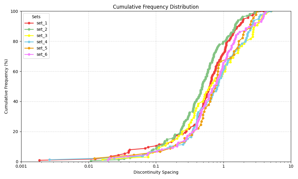 The cumulative frequency distribution of spacings for each set.
Looking at the cumulative spacing distribution of set 2, we can see that it contains a higher proportion of smaller spacings compared to the other sets. This is also reflected in the smallest median spacing of 0.49 m reported in the statistics table.
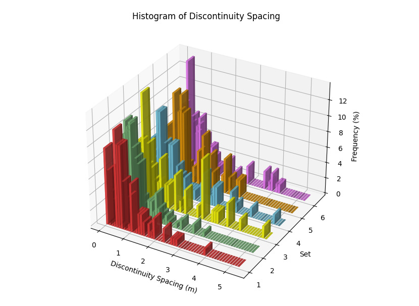 Histogram of discontinuity spacing for each set.
In the histogram of discontinuity spacings, we again observe a general trend toward smaller spacings across all sets. In set 3, however, a secondary peak appears around 3 m, accounting for approximately 6% of the measured spacings. This feature is also visible in the cumulative frequency distribution, where it produces a pronounced steep section of the curve at around 3 m spacing.
The following references provide additional details on the computational methods, if you are interested in how the calculations are performed:
Riquelme, A.J., Abellan, A., Tomas, R., Jaboyedoff, M. (2014): A new approach for semi-automatic rock mass joints recognition from 3D point clouds. Computers & Geosciences, 68, 38-52. https://www.sciencedirect.com/science/article/pii/S0098300414000740
Riquelme, A.J., Abellan, A., Tomas, R. (2015): Discontinuity spacing analysis in rock masses using 3D point clouds. Engineering Geology, 195, 185-195. https://www.sciencedirect.com/science/article/abs/pii/S0013795215002045
Wichmann, V., Strauhal, T., Fey, C., Perzlmaier, S. (2019): Derivation of space-resolved normal joint spacing and in situ block size distribution data from terrestrial LIDAR point clouds in a rugged Alpine relief (Kuehtai, Austria). Bulletin of Engineering Geology and the Environment, 78, 4465-4478. https://doi.org/10.1007/s10064-018-1374-7