TLS-Forestry Tree Architecture Tutorial
Learn how to extract forestry related metrics such as single tree diameters, tree heights, crown radii and wood volume from LiDAR point clouds.
Contents
- Dataset Visualization
- Ground Classification
- Stem Diameter Extraction (DBH)
- Tree Segmentation
- Tree Architecture
- Automation
The Dataset
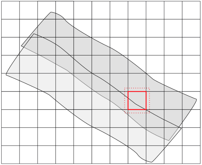
The dataset is a small extract from a mountainous beech forest stand, located at the edge of the forest. It has been selected for this tutorial as it is challenging to analyze because of its characteristics (dense growth, understory, hillside situation). It was acquired by terrestrial laserscanning (TLS). In order to be able to reconstruct the tree architecture, we require both a highly-detailed point cloud as well as intensity/reflectance values for each point. Thus, in most cases such a reconstruction will require a close-range LiDAR point cloud like used in this tutorial (the data of this tutorial was acquired with a Riegl VZ 2000i instrument).
The default parameter values of the tree segmentation and reconstruction tools are optimized for TLS point clouds. In case of e.g. uncrewed laserscanning (ULS), mobile laserscanning (MLS) or even high density airborne laserscanning (ALS), some of the values (e.g. the search radius) have to be increased in order to adjust the tools to the lower point density of such datasets.
Data Download
You can download the tutorial dataset here
Prerequisites
Please note that some steps in this tutorial require the LIS Pro 3D Forestry Addon if you want to process the data yourself.
Data Description
The tutorial dataset is provided as a SAGA point cloud (*.sg-pts-z) and has the following attributes:
x,y,z-coordinates
intensity (reflectance)
deviation (pulse shape deviation of the laser return, compared to the outgoing laser pulse)
The pulse shape deviation attribute is not mandatory for the processing pipeline shown in this tutorial, but it improves the result. Both intensity and deviation are used to detect branches.
LIS Pro 3D offers options to start the processing from other common file formats like LAS/LAZ or Riegl RDB as well.
Load and Visualize the Point Cloud
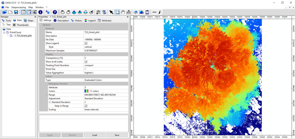
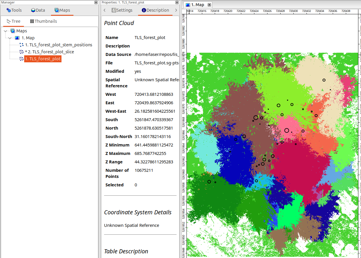
Let’s start by opening LIS Pro 3D. Load the “TLS_forest_plot.sg-pts-z” point cloud via the “File > Point Cloud > Load” menu (or simply drag and drop the file into the GUI).
A double-click on the dataset in the Data tab of the Manager window shows the point cloud in a Map View.
We recommend creating a SAGA GIS project when starting a new workflow. Regularly saving the project and any processed data (vector and raster datasets, as well as point clouds) can also be very helpful.
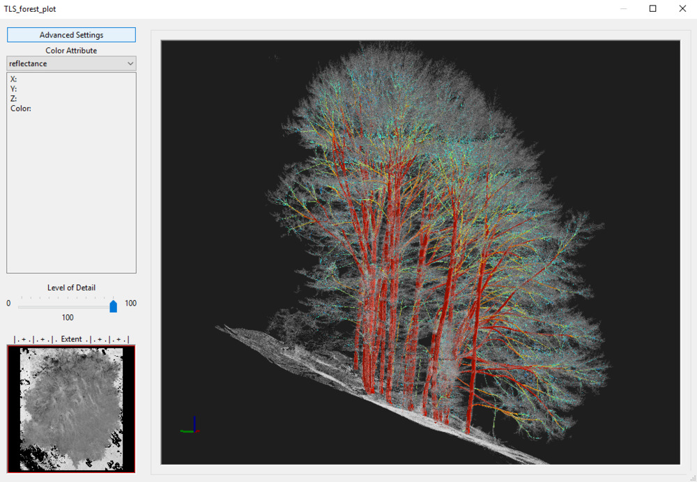
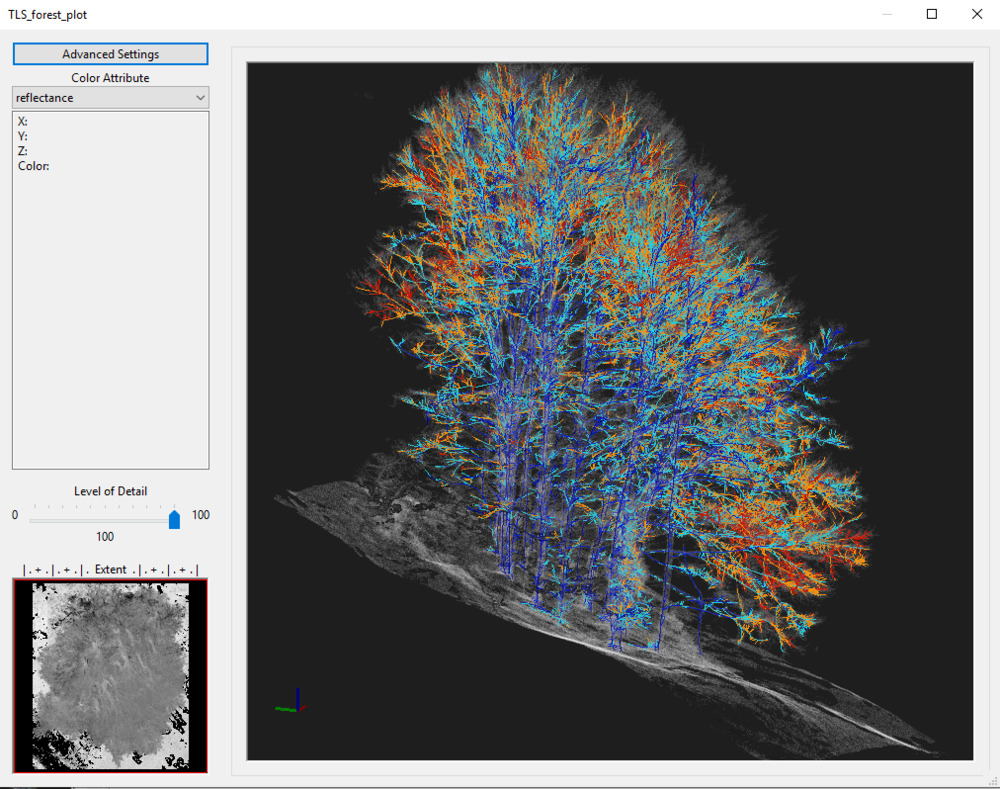
3D Visualization
Open the Point Cloud Editor. Provide the point cloud as input and pass the “reflectance” attribute with the “Intensity” parameter. This will enable us to use the keyboard shortcut “2” to switch to reflectance visualization. Also pass the “reflectance” and “deviation” as report attributes. This will allow us to view these values on “mouse over”.
In all our tutorials, we describe the execution of individual tools via the Tool Libraries interface. If you are not familiar with executing tools this way, please consult this section in our introductory tutorial series. In this section, we describe how you can locate the tools in LIS Pro 3D’s GUI.
Tool: Point Cloud Editor
Geoprocessing: LIS Pro 3D → Point Cloud Editor // Tools → LIS Pro 3D → Point Cloud Editor
| Parameter | Setting |
|---|---|
| Data Objects | |
| Point Clouds | |
| >> Point Cloud | TLS_forest_plot |
| Intensity | reflectance |
| RGB | <not set> |
| Shading | <not set> |
| Classification | <not set> |
| Random | <not set> |
| Normal Vector (X) | <not set> |
| Report Attribute 1 | reflectance |
| Report Attribute 2 | deviation |
| Grids | |
| > Elevation Grids | No objects |
| > Color Grids | No objects |
| Shapes | |
| > Shapes | <not set> |
| Options | |
| Work on Copy of Point Cloud | ☐ |
| Background Color | Black |
Execute the tool.
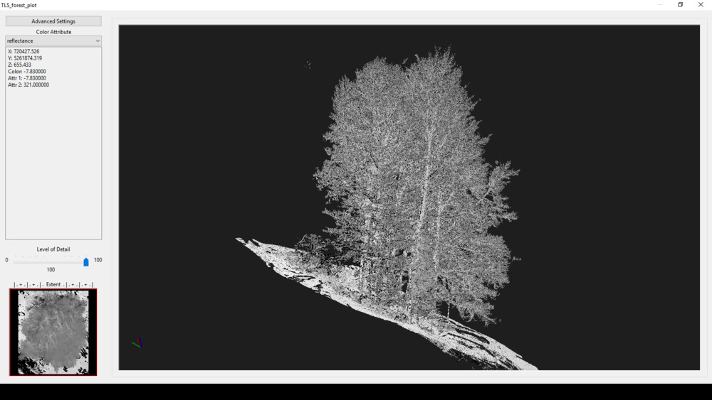
Press shortcut key “2” to switch from elevation to intensity colored (use shortcut key “1” if you want to switch back to elevation). Hover the mouse over the main branches of the trees and read out some “reflectance” (Attr. 1) and “deviation” (Attr. 2) values reported in the text box. We will use these values for filtering later. Finally quit the Point Cloud Editor by simply closing its window.
Ground Classification
A prerequisite for all further analyses is the classification of ground points and the calculation of the “height above ground” for each point (“point cloud normalization”). This can be done in a single step using the Ground Classification tool. Run the tool with the following parameters:
Tool: Ground Classification
Geoprocessing: LIS Pro 3D → Classification // Tools → LIS Pro 3D → Classification
| Parameter | Setting |
|---|---|
| Data Objects | |
| Point Clouds | |
| >> Point Cloud | TLS_forest_plot |
| Classification | <not set> |
| Segment ID | <not set> |
| Copy existing attributes | 🗹 |
| Spatial Sorting | ☐ |
| < Point Cloud Classified | <not set> |
| Attribute Suffix | |
| < TIN Polygons | <not set> |
| Options | |
| Seed Generation | |
| Initial Cellsize | 50 |
| Final Cellsize | 1 |
| Adjust Cellsize | ☐ |
| Filter Seeds | ☐ |
| TIN Densification | |
| Terrain Angle | 88 |
| Minimum Edge Length | 0.5 |
| Maximum Angle | 25 |
| Maximum Distance | 0.8 |
| Z Tolerance | 0.05 |
| Segments | |
| Point Cloud Normalization | |
| Attach DZ to Point Cloud | 🗹 |
| Classification |
Provide the point cloud as input. We can use the default parameter settings for the ground seed generation. As the plot is located on a hillside, we reduce the “Minimum Edge Length” to 0.5 (m) and increase the “Maximum Angle” to 25°. With the “Attach DZ to Points” parameter checked, the tool will not only classify the ground points but will also calculate the height above ground for each point.
After execution, the point cloud has been updated and has been extended by 2 attributes: “grdclass” and “dz”.
3D Visualization of the Classification Result
Change back to the Point Cloud Editor and pass the new “grdclass” attribute with the “Classification” parameter to the Point Cloud Editor.
Tool: Point Cloud Editor
Geoprocessing: LIS Pro 3D → Point Cloud Editor // Tools → LIS Pro 3D → Point Cloud Editor
| Parameter | Setting |
|---|---|
| Data Objects | |
| Point Clouds | |
| >> Point Cloud | TLS_forest_plot |
| Intensity | reflectance |
| RGB | <not set> |
| Shading | <not set> |
| Classification | grdclass |
| Random | <not set> |
| Normal Vector (X) | <not set> |
| Report Attribute 1 | reflectance |
| Report Attribute 2 | deviation |
| Grids | |
| > Elevation Grids | No objects |
| > Color Grids | No objects |
| Shapes | |
| > Shapes | <not set> |
| Options | |
| Work on Copy of Point Cloud | ☐ |
| Background Color | Black |
| Classification LUT | ASPRS LAS (Formats 6-10) |
- Click Execute
This will enable us to use the keyboard shortcut “5” to switch to the visualization of the classification.
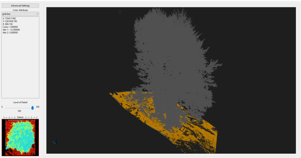
Press shortcut key “5” to switch from elevation to classification colored (use shortcut key “6” if you want to visualize only the points classified as ground).
Tree Trunk and DBH detection
Now, we would like to extract tree trunks and DBH via the Tree Trunk and DBH Detection tool. Open the tool and set the following parameters:
Tool: Tree Trunk and DBH Detection
Geoprocessing: LIS Pro 3D → Forestry → Point Cloud // Tools → LIS Pro 3D → Forestry
| Parameter | Setting |
|---|---|
| Data Objects | |
| Point Clouds | |
| >> Point Cloud | TLS_forest_plot |
| DZ | dz |
| Tree Height | <not set> |
| Intensity | reflectance |
| Deviation | deviation |
| Copy existing Attributes | 🗹 |
| Options | |
| Output Stems | |
| << Output Stem Positions | <create> |
| < Point Cloud Slice | <create> |
| Attribute Suffix | |
| Stem Detection | |
| Method Stem Detection | single slice |
| DBH Slice Height | 1.3 |
| DBH Slice Thickness | 0.1 |
| Minimum Intensity | -8 |
| Maximum Deviation | 14 |
| Search Radius | 0.1 |
| Minimum Point Count | 30 |
| Minimum Compactness | 70 |
| Stem Diameter Estimation | |
| Stem Diameter Range | 0.05;0.6 |
| Circle Fitting Tolerance | 12.5 |
| Filtering | |
| Points on Circle | 10 |
| Goodness of Fit | 80 |
| Circle Completeness | 40 |
| Percentile Radius | 25 |
| Apply Correction Function | ☐ |
- Click Execute
Visualize Estimated Tree Trunk Diameters
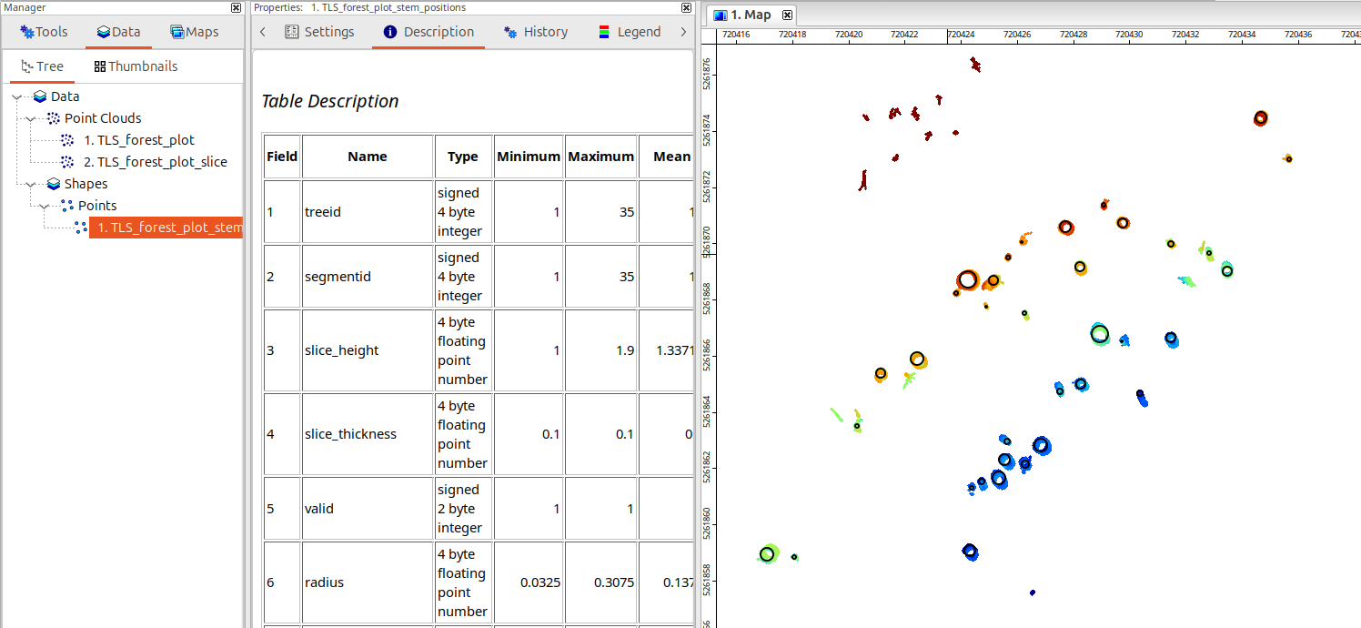
A new point cloud slice and tree positions have been detected. Do a double-click on the new “TLS_forest_plot_slice” point cloud in the Data tab and add it to the existing Map View.
Also add the new “TLS_forest_plot_stem_positions” point dataset to the same Map View. Then adjust the settings for fill Style, Outline and Size as follows:
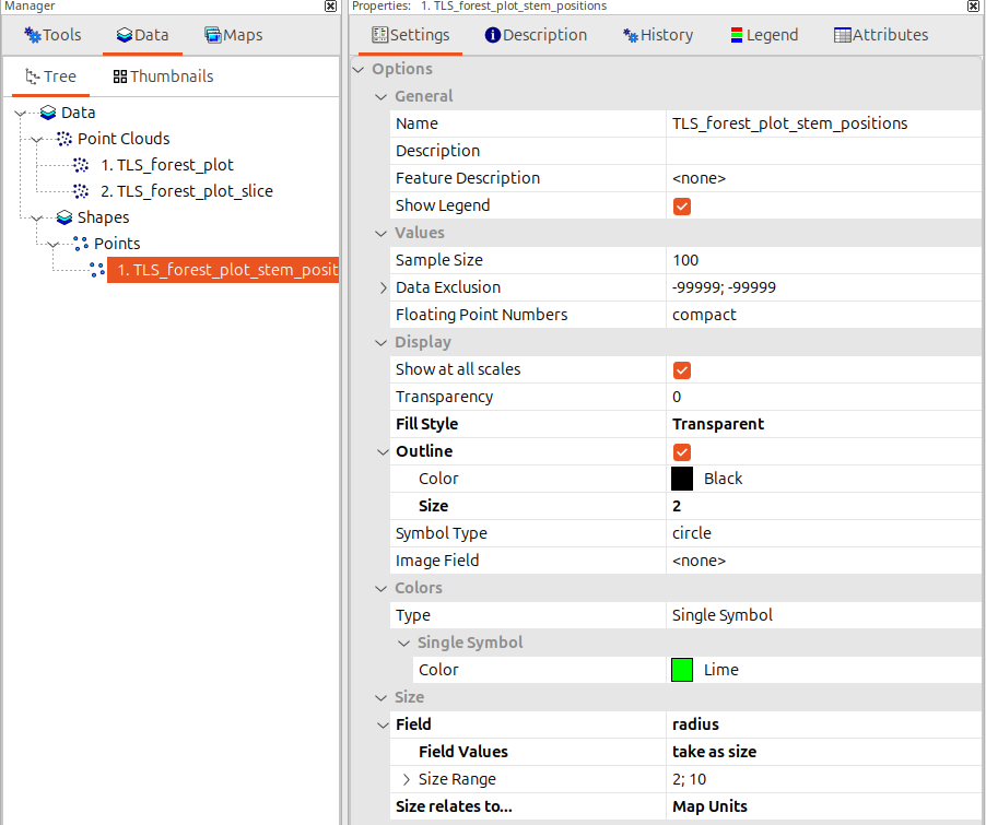
Then apply the changes (“Apply” button).
These settings will render the points in the size of the estimated trunk radius.
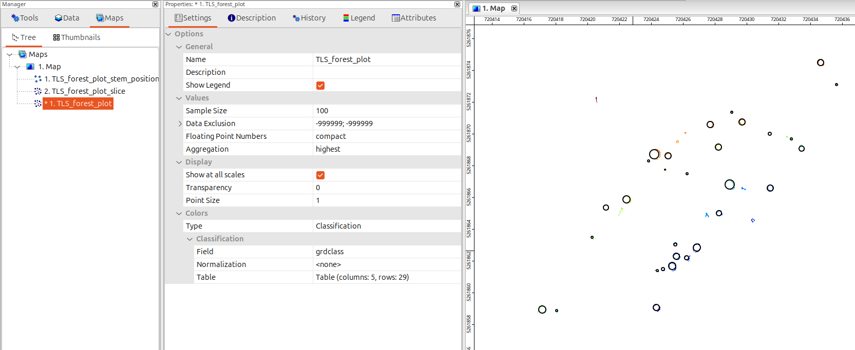
Change to the Maps tab. Double-clicking on the “TLS_forest_plot_stem_positions” point dataset will toggle the rendering of this map layer on and off. This way you can compare the fitted circles and their diameters with the point cloud data.
Tree Trunk and DBH Detection (multi slice)
In some situations, especially when dense understory is present in the scanned plot, it might be helpful to detect the tree trunks using multiple height slices. In this case the best detection (highest circle completeness, goodness of fit, etc.) will be used as the stem postion of a trunk. This height might differ from the the exact breast height definition and represents a single slice in the selected height range for multi slice picking.
Now execute the tool again, but make sure to adjust the parameters as follows, the outputs will be updated (i.e., previous output will be overwritten):
Tool: Tree Trunk and DBH Detection
Geoprocessing: LIS Pro 3D → Forestry → Point Cloud // Tools → LIS Pro 3D → Forestry
| Parameter | Setting |
|---|---|
| Data Objects | |
| Point Clouds | |
| >> Point Cloud | TLS_forest_plot |
| DZ | dz |
| Tree Height | <not set> |
| Intensity | reflectance |
| Deviation | deviation |
| Copy existing Attributes | 🗹 |
| Options | |
| Output Stems | |
| << Output Stem Positions | TLS_forest_plot_stem_positions |
| < Point Cloud Slice | TLS_forest_plot_slice |
| Attribute Suffix | |
| Stem Detection | |
| Method Stem Detection | multiple slices |
| DBH Slice Height Range | 1;2 |
| DBH Slice Stepping | 0.1 |
| Slice Connection Distance | 0.1 |
| DBH Slice Thickness | 0.1 |
| Minimum Intensity | -8 |
| Maximum Deviation | 14 |
| Search Radius | 0.1 |
| Minimum Point Count | 30 |
| Minimum Compactness | 70 |
| Stem Diameter Estimation | |
| Stem Diameter Range | 0.05;0.6 |
| Circle Fitting Tolerance | 12.5 |
| Filtering | |
| Points on Circle | 10 |
| Goodness of Fit | 80 |
| Circle Completeness | 40 |
| Minimum Detections per Stem | 2 |
| Percentile Radius | 25 |
| Apply Correction Function | ☐ |
The operation takes longer than single slice mode as multiple slices are analysed.
In the “Stem Detection” Parameters, select the “multiple slices” method and define the height above ground range (DBH Slice Height Range: 1;2m) and a “DBH Slice Stepping” (0.1m). In this case 11 vertically stacked slices will be analysed.
This allows detecting more stems. As at a single slice height a tree might be occluded by understory, we have a chance to detect it on a higher or lower height slice.
Additionally, setting the “Minimum Detections per Stem” to 2 will only accept a tree trunk if it is at least detected on two slice height levels. This is helpful in order to suppress false detections in understory.
In the Maps View, you can now see the thicker point cloud slice used for circle detection. For the 11 analysed slice heights, the slice with the best fitting stats is used in order to define the stem position and diameter.
Segmentation of Individual Trees
LASERDATA LiS > Forestry > 3D Single Tree Derivation
Now we will extract single trees from the 3D point cloud using the Single Tree Derivation 3D tool with the following settings:
Tool: Single Tree Derivation 3D
Geoprocessing: LIS Pro 3D → Forestry → Point Cloud // Tools → LIS Pro 3D → Forestry
| Parameter | Setting |
|---|---|
| Data Objects | |
| Point Clouds | |
| >> Point Cloud | TLS_forest_plot |
| Intensity | reflectance |
| Deviation | deviation |
| Classification | grdclass |
| DZ | dz |
| Copy existing attributes | 🗹 |
| Exclude Point Classes | 2;6;9 |
| Shapes | |
| > Known Tree Positions | TLS_forest_plot_stem_positions |
| Tree ID | treeid |
| DBH | diameter_mean |
| Slice Height | slice_height |
| Seed Blocking Distance | <not set> |
| Initial Gap Size | <not set> |
| Synthetic Stem Height | <not set> |
| Grids | |
| Grid system | <not set> |
| > Seed Mask | <not set> |
| Options | |
| Output | |
| < Point Cloud Segmented | <not set> |
| Attribute Suffix | |
| << Tree Positions | <create> |
| Segmentation | |
| Step Size | 0.5 |
| Cost Weighting | 1.5 |
| Maximum Gap Size | 0.3 |
| Foliage Label Distance | 2 |
| Minimum Intensity | -7 |
| Maximum Deviation | 14 |
| Minimum Point Density | 0 |
| Minimum Tree Height | 5 |
| Crown Metrics Resolution | 0.1 |
| Iterations | 1 |
| Output All Trees | 🗹 |
| Shift Synthetic Seeds to Crown Center | ☐ |
| Start Cost Synthetic Seeds | 0 |
| Automation | |
| Specify Tile Origin | ☐ |
Provide the point cloud as input and pass the “reflectance”, “deviation”, “grdclass” and “dz” attribute fields.
We provide the “TLS_forest_plot_stem_positions” dataset from the previous processing step to the “Know Tree Positions” parameter and set the “Tree ID”, “DBH” and “Slice Height” attributes. These settings will use the stem positions as seed points and will create additional seed points for every 0.5m (“Step Size” parameter).
We set the “Cost Weighting” to 1.5. The smaller this value, the better the segmentation of tilted trees. Higher values improve the segmentation of tall trees. Set the “Maximum Gap Size” to 0.3, this parameter should be set to about the size of the largest data gap within the point cloud. Set the “Foliage Label Distance” to 2m. As the segmentation is based on the main branches, this parameter controls how tolerantly foliage is added to the single tree segments.
Set the “Minimum Tree Height” parameter to e.g. 5m. This will ignore all output tree segments with trees smaller than 5m. Check “Output All Trees”. In this case, also tree segments are written to the output, where no diameter could be found. Otherwise only tree segments with valid trunk diameters are written to the output.
After tool execution the point cloud shows a random color for each tree segment (so this may look slightly different to the example here!).
Note, that a tree_positions file has been created. This file stores the basic tree informations in its attribute table (treeid, dbh, tree_height, crown_diameter,…)
You can add the newly created “tree_positions” point dataset (yellow points) to the Map View. The tree positions are used as seed points for the next processing step.
3D Visualization of the Tree Segmentation
We choose the following settings for visualizing the individual tree segments:
Tool: Point Cloud Editor
Geoprocessing: LIS Pro 3D → Point Cloud Editor // Tools → LIS Pro 3D → Point Cloud Editor
| Parameter | Setting |
|---|---|
| Data Objects | |
| Point Clouds | |
| >> Point Cloud | TLS_forest_plot |
| Intensity | reflectance |
| RGB | <not set> |
| Shading | <not set> |
| Classification | grdclass |
| Random | treeid |
| Normal Vector (X) | <not set> |
| Report Attribute 1 | reflectance |
| Report Attribute 2 | deviation |
| Grids | |
| > Elevation Grids | No objects |
| > Color Grids | No objects |
| Shapes | |
| > Shapes | <not set> |
| Options | |
| Work on Copy of Point Cloud | ☐ |
| Background Color | Black |
| Classification LUT | ASPRS LAS (Formats 6-10) |
This will enable us to use the keyboard shortcut “q” to colorize each tree by a random color.
- Click Execute
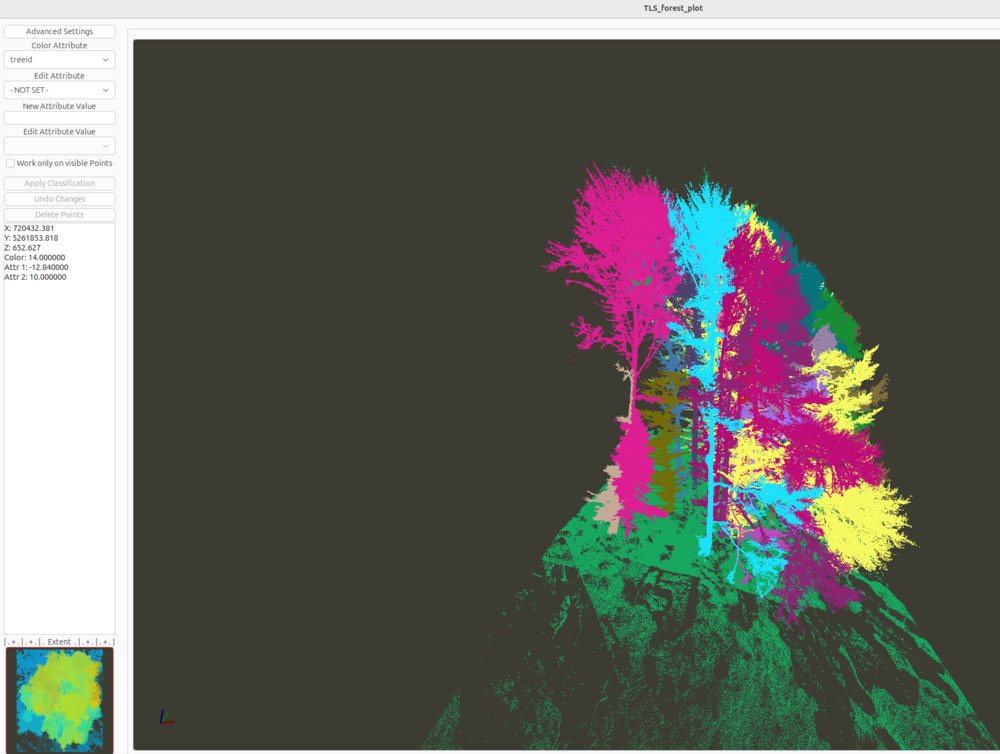
Press shortcut key “q” to switch from elevation to random colored. Press “q” again to get another color palette. Each tree segment now has its own color.
Note that a tree ID of “0” labels undefined segments (like the ground).
Press “Alt + q” repeatedly to visualize the segments one by one (press “q” to show all segments again). You can change from central to parallel perspective rendering with shortcut key “p”. When finished with the visual inspection, close the point cloud editor to continue with the next steps.
Tree Metrics
Now we have prepared all data required to reconstruct the tree architecture. Use the following tool and parameters to calculate branching parameters as well as wood volume:
Tool: Tree Shape Metrics 3D
Geoprocessing: LIS Pro 3D → Forestry → Point Cloud // Tools → LIS Pro 3D → Forestry
| Parameter | Setting |
|---|---|
| Data Objects | |
| Point Clouds | |
| >> Point Cloud | TLS_forest_plot |
| Intensity | reflectance |
| Deviation | deviation |
| Tree ID | treeid |
| Copy Existing Attributes | 🗹 |
| < Point Cloud | <not set> |
| Attribute Suffix | |
| Shapes | |
| >> Seeds | TLS_forest_plot_tree_positions |
| Seed ID | treeid |
| DBH | dbh |
| Slice Height | <not set> |
| Diameter Factor | 1.5 |
| > Stem Axes | <not set> |
| << Tree Metrics | <create> |
| Options | |
| Intensity and Deviation Processing | |
| Minimum Intensity Value | -7 |
| Maximum Deviation Value | 14 |
| Value Range Normalization | -7;0 |
| Scale Factor | 4 |
| Region Growing | |
| Search Radius | 0.1 |
| Bridge Distance | 0.5 |
| Iterations | 10 |
| Skeletonization | |
| Node Stepping | 0.2 |
| Branching Distance | 0.1 |
| < Skeleton | <create> |
| < Simplified Skeleton | <not set> |
| < Pipe Model | <create> |
| Number of Prism Faces | 5 |
| Branch Radius | pipe model approach |
| < Diameter Rings | <not set> |
| Minimum Number of Children | 10 |
| Minimum Modelling Diameter | 0.02 |
| Fork Ratio | 90 |
| Minimum Fork Diameter | 0.15 |
| Sigma (Smoothing) | 2 |
| Direction Detection Length | 1 |
| Model Fine Adjustment | |
| Adjustment Mode | no adjustment |
| Adjustment - Circle Fitting Parameters | |
| Log Classification | |
| Long Log Classification | leave as is |
Provide the point cloud as well as the tree positions dataset as input and pass the required attribute fields. Intensity and deviation parameters are again used to detect main branches.
The “Region Growing” parameters control the path finding of the branches geometrically . The “Search Radius” is used to find neighboring points. The “Bridge Distance” should be as large as the largest gap in the data (the tool performs an iterative growing: as soon as no more neighbors are found within the search radius, the bridge distance is applied and a new growing iteration is started).
The “Skeletonization” parameters control the detail of the optional vector output datasets: the skeleton (3D lines) as well as a pipe model (3D polygons) of each tree. Increase the “Node Stepping” to 0.2 (m) and “Branching Distance” to 0.1 (m) For the visualization of the tree models, set the “Number of Prism Faces” to 5.
The tool creates three new datasets:
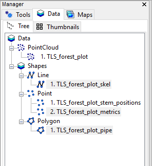
- a point vector dataset (“TLS_forest_plot_metrics”), which summarizes and aggregates the calculation results for each tree; the derived metrics are shown further below.
- a 3D line vector dataset (“TLS_forest_plot_skel”) with the tree skeletons
- a 3D polygon vector dataset (“TLS_forest_plot_pipe”) with the derived pipe model
All datasets provide valuable attributes derived from the reconstructed tree architecture. Some attributes are also attached to the input point cloud.
When you select a dataset you can have a look at the Description tab of the Properties window to see which attributes are available:
| Attribute | Description |
|---|---|
| TreeID: | ID of the given tree (automatically assigned during processing) |
| DBH: | Diameter at breast height |
| CrownRadius: | Radius of the delineated crown |
| CrownArea: | 2D footprint area of the tree crown |
| TreeHeight: | Tree height |
| CrownBottom: | Height (of the lowest point) of the lowest first order branch with a minimum number of children |
| GroundHeight: | Ground elevation at the tree position |
| MaxHierarchy: | Maximum value of the hierarchical levels detected; shows the complexity of a tree |
| WoodVolume: | Total wood volume of the tree |
| WoodVolume0: | Total wood volume of hierarchical level 0 (the trunk) of the tree |
| WoodVolume1: | Total wood volume of hierarchical level 0 and 1 of the tree |
| WoodVolume10cm: | Total wood volume up to a branch diameter of 10 cm |
| WoodVolume6cm: | Total wood volume up to a branch diameter of 6 cm |
| WoodVolume4cm: | Total wood volume up to a branch diameter of 4 cm |
| AverageBranchingAngle: | Average angle of branches (tree trunk of a spruce tree = 90°, branches of a spruce tree often show angles ≤ 0°) |
| AverageDifferenceAngle: | Average of the angle difference between child branches and their parent branches (for coniferous trees the angle between trunk and first order branches is ≥ 90°, for deciduous trees it is often smaller) |
| NumBranches: | Total number of branches within the tree topology; should be related to tree height and age |
| NumFirstOrderBranches: | Total number of branches connected to the tree trunk; should be related to tree height and age |
| Fork: | Indicates if a Fork was found in the branching structure |
| ForkX: | X-Coordinate of the Fork Location (if fork was found) |
| ForkY: | Y-Coordinate of the Fork Location (if fork was found) |
| ForkZ: | Z-Coordinate of the Fork Location (if fork was found) |
| ForkAngle: | The angle between the two forking trunks (if fork was found) |
(there are a few more attributes that are not listed here)
View Tree Metrics
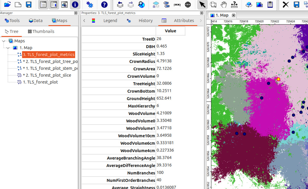
Add the point vector dataset “TLS_forest_plot_metrics” to the Map View and select one of the points with the Action tool (the black arrow in the tool bar).
The dataset to select from must be selected in the Data tab or Map tab in order to perform selections.
Change to the Attributes tab of the Properties window to get the aggregated metrics for the selected tree reported:
You may have noticed that the “TLS_forest_plot_metrics” contains less points (trees) than the initial “TLS_forest_plot_stem_positions” dataset. This is because some trees smaller than 5m have already been filtered out (see Segmentation of individual Trees).
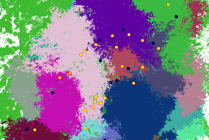
Selecting Trees with Specific Characteristics
The map below shows a selection of trees larger than 15m. You can do such selections with the Select by Attributes… (Numerical Expression) tool:
Tool: Select by Attributes… (Numerical Expression)
Geoprocessing → Shapes → Selection // Tools → Shapes → Tools
| Parameter | Setting |
|---|---|
| Data Objects | |
| Shapes | |
| >> Shapes | TLS_forest_plot_metrics |
| Attribute | TreeHeight |
| Options | |
| Expression | a > 15 |
| Inverse | ☐ |
| Use No-Data | ☐ |
| Method | new selection |
| Post Job | none |
If desired, you may also copy this selection to a new layer using the Copy Selection to New Shapes Layer” tool.
3D Visualization of the Pipe Models
We can use the “3D Shapes Viewer” tool to have a look at the created pipe models with the following parameters:
Tool: 3D Shapes Viewer
Geoprocessing: Visualization → 3D Viewer // Tools → Visualization → 3D Viewer
| Parameter | Setting |
|---|---|
| Data Objects | |
| Shapes | |
| >> Shapes | TLS_forest_plot_pipe |
| Colour | RadiusModel |
- Click Execute
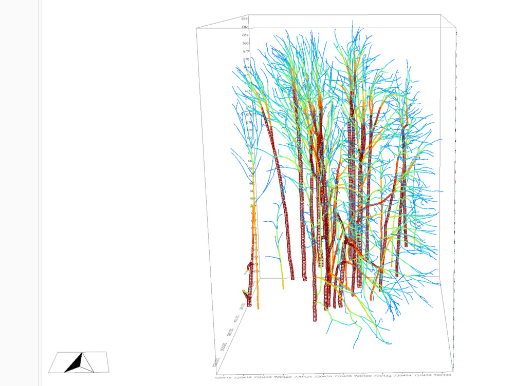
This shows the pipe models created from the processed point cloud data, colored by branch radius. When finished with the visual inspection, close the point cloud editor to continue.
We can also have a look at the pipe models together with the point cloud in the “Point Cloud Editor” using the following settigns:
Tool: Point Cloud Editor
Geoprocessing: LIS Pro 3D → Point Cloud Editor // Tools → LIS Pro 3D → Point Cloud Editor
| Parameter | Setting |
|---|---|
| Data Objects | |
| Point Clouds | |
| >> Point Cloud | TLS_forest_plot |
| Intensity | reflectance |
| RGB | <not set> |
| Shading | <not set> |
| Classification | grdclass |
| Random | treeid |
| Normal Vector (X) | <not set> |
| Report Attribute 1 | reflectance |
| Report Attribute 2 | deviation |
| Grids | |
| > Elevation Grids | No objects |
| > Color Grids | No objects |
| Shapes | |
| > Shapes | TLS_forest_plot_pipe |
| Color | RadiusModel |
| Options | |
| Work on Copy of Point Cloud | ☐ |
| Background Color | Black |
| Classification LUT | ASPRS LAS (Formats 6-10) |
3D Visualization of the Tree Skeletons
We can also have a look at the derived tree skeletons in the “Point Cloud Editor”. To do so, simply change the shapes and the attribute in the editor as follows:
Tool: Point Cloud Editor
Geoprocessing: LIS Pro 3D → Point Cloud Editor // Tools → LIS Pro 3D → Point Cloud Editor
| Parameter | Setting |
|---|---|
| … | … |
| Shapes | |
| > Shapes | TLS_forest_plot_skel |
| Color | Hierarchy |
| … | … |
Starting the editor will show a picture similar to this:
Press shortcut key “2” to switch to intensity colored. Use “F11/F12” to control the point cloud transparency.
Automated Processing
The processing pipeline can be automated in several ways. Besides classic batch processing, LIS Pro 3D supports Python scripting with the PySAGA Python Interface. This allows for full control as you can execute and chain tools as well as compute stuff with the SAGA C++ functions wrapped into Python.
For simpler usage, LASERDATA also provides a dedicated (C++) tool library for automation. In this library, the tools used in this tutorial are wrapped into “meta tools” that allow you to run each tool on a user-defined tiling scheme (and thus on point clouds covering a large area) without additional scripting.